
Negative Metric Learning for Graphs
Proceedings of the Thirty-Fourth International Joint Conference on Artificial Intelligence. Main Track. Pages 7137-7145.
https://doi.org/10.24963/ijcai.2025/794
Keywords
- Machine Learning: ML: Sequence and graph learning
- Machine Learning: ML: Self-supervised Learning
Abstract
Graph contrastive learning (GCL) often suffers from false negatives, which degrades the performance on downstream tasks. The existing methods addressing the false negative issue usually rely on human prior knowledge, still leading GCL to suboptimal results. In this paper, we propose a novel Negative Metric Learning (NML) enhanced GCL (NML-GCL). NML-GCL employs a learnable Negative Metric Network (NMN) to build a negative metric space, in which false negatives can be distinguished better from true negatives based on their distance to anchor node. To overcome the lack of explicit supervision signals for NML, we propose a joint training scheme with bi-level optimization objective, which implicitly utilizes the self-supervision signals to iteratively optimize the encoder and the negative metric network. The solid theoretical analysis and the extensive experiments conducted on widely used benchmarks verify the superiority of the proposed method.
- [Campello, 2007] Ricardo JGB Campello. A fuzzy extension of the rand index and other related indexes for clustering and classification assessment. Pattern Recognition Letters, 28(7):833-841, 2007.
- [Chi and Ma, 2024] Hongliang Chi and Yao Ma. Enhancing contrastive learning on graphs with node similarity. In Pro- ceedings of the 30th ACM SIGKDD Conference on Knowl- edge Discovery and Data Mining, pages 456-465, 2024.
- [Chuang et al., 2020] Ching-Yao Chuang, Joshua Robinson, Yen-Chen Lin, Antonio Torralba, and Stefanie Jegelka. Debiased contrastive learning. Advances in neural infor- mation processing systems, 33:8765-8775, 2020.
- [Fan et al., 2023] Lu Fan, Jiashu Pu, Rongsheng Zhang, and Xiao-Ming Wu. Neighborhood-based hard negative min- ing for sequential recommendation. In Proceedings of the 46th International ACM SIGIR Conference on Research and Development in Information Retrieval, pages 2042- 2046, 2023.
- [Han et al., 2023] Lei Han, Hui Yan, and Zhicheng Qiao. Topology-aware debiased self-supervised graph learning for recommendation. In 2023 IEEE International Con- ference on Systems, Man, and Cybernetics (SMC), pages 2339-2344. IEEE, 2023.
- [Hao et al., 2024] Zhezheng Hao, Haonan Xin, Long Wei, Liaoyuan Tang, Rong Wang, and Feiping Nie. Towards expansive and adaptive hard negative mining: Graph con- trastive learning via subspace preserving. In Proceedings of the ACM on Web Conference 2024, 2024.
- [Hassani and Khasahmadi, 2020] Kaveh Hassani and Amir Hosein Khasahmadi. Contrastive multi-view repre- sentation learning on graphs. In International conference on machine learning, pages 4116-4126. PMLR, 2020.
- [Hu et al., 2021] Yang Hu, Haoxuan You, Zhecan Wang, Zhicheng Wang, Erjin Zhou, and Yue Gao. Graph-mlp: Node classification without message passing in graph. arXiv preprint arXiv:2106.04051, 2021.
- [Huynh et al., 2022] Tri Huynh, Simon Kornblith, Matthew R Walter, Michael Maire, and Maryam Khademi. Boosting contrastive self-supervised learning with false negative cancellation. In Proceedings of the IEEE/CVF winter conference on applications of computer vision, pages 2785-2795, 2022.
- [Kipf and Welling, 2017] Thomas N. Kipf and Max Welling. Semi-supervised classification with graph convolutional networks. In International Conference on Learning Rep- resentations, 2017.
- [Li et al., 2023] Wen-Zhi Li, Chang-Dong Wang, Hui Xiong, and Jian-Huang Lai. Homogcl: Rethinking ho- mophily in graph contrastive learning. In Proceedings of the 29th ACM SIGKDD Conference on Knowledge Dis- covery and Data Mining, pages 1341-1352, 2023.
- [Lin et al., 2022] Shuai Lin, Chen Liu, Pan Zhou, Zi-Yuan Hu, Shuojia Wang, Ruihui Zhao, Yefeng Zheng, Liang Lin, Eric Xing, and Xiaodan Liang. Prototypical graph contrastive learning. IEEE transactions on neural net- works and learning systems, 35(2):2747-2758, 2022.
- [Liu et al., 2022] Yixin Liu, Ming Jin, Shirui Pan, Chuan Zhou, Yu Zheng, Feng Xia, and S Yu Philip. Graph self-supervised learning: A survey. IEEE transactions on knowledge and data engineering, 35(6):5879-5900, 2022.
- [Liu et al., 2023] Mengyue Liu, Yun Lin, Jun Liu, Bohao Liu, Qinghua Zheng, and Jin Song Dong. B2-sampling: Fusing balanced and biased sampling for graph contrastive learning. In Proceedings of the 29th ACM SIGKDD Con- ference on Knowledge Discovery and Data Mining, pages 1489-1500, 2023.
- [Liu et al., 2024] Xin Liu, Biao Qian, Haipeng Liu, Dan Guo, Yang Wang, and Meng Wang. Seeking false hard negatives for graph contrastive learning. IEEE Transac- tions on Circuits and Systems for Video Technology, 2024.
- [Mernyei and Cangea, 2020] Péter Mernyei and Cȃtȃlina Cangea. Wiki-cs: A wikipedia-based benchmark for graph neural networks. arXiv preprint arXiv:2007.02901, 2020.
- [Niu et al., 2024] Chaoxi Niu, Guansong Pang, and Ling Chen. Affinity uncertainty-based hard negative mining in graph contrastive learning. IEEE Transactions on Neural Networks and Learning Systems, 2024.
- [Poole et al., 2019] Ben Poole, Sherjil Ozair, Aaron Van Den Oord, Alex Alemi, and George Tucker. On variational bounds of mutual information. In International Confer- ence on Machine Learning, pages 5171-5180. PMLR, 2019.
- [Rong et al., 2020] Yu Rong, Wenbing Huang, Tingyang Xu, and Junzhou Huang. Dropedge: Towards deep graph con- volutional networks on node classification. In Interna- tional Conference on Learning Representations, 2020.
- [Shchur et al., 2018] Oleksandr Shchur, Maximilian Mumme, Aleksandar Bojchevski, and Stephan Günnemann. Pitfalls of graph neural network evalu- ation. Relational Representation Learning Workshop, NeurIPS 2018, 2018.
- [Steinley, 2004] Douglas Steinley. Properties of the hubert- arable adjusted rand index. Psychological methods, 9(3):386, 2004.
- [Sun et al., 2023] Qingqiang Sun, Wenjie Zhang, and Xuemin Lin. Progressive hard negative masking: From global uniformity to local tolerance. IEEE Transactions on Knowledge and Data Engineering, 35(12):12932-12943, 2023.
- [Thakoor et al., 2021] Shantanu Thakoor, Corentin Tallec, Mohammad Gheshlaghi Azar, Remi Munos, Petar Veličković, and Michal Valko. Bootstrapped representa- tion learning on graphs. In ICLR 2021 Workshop on Geo- metrical and Topological Representation Learning, 2021.
- [Veličković et al., 2018] Petar Veličković, William Fedus, William L Hamilton, Pietro Liò, Yoshua Bengio, and R Devon Hjelm. Deep graph infomax. arXiv preprint arXiv:1809.10341, 2018.
- [Wan et al., 2023] Sheng Wan, Yibing Zhan, Shuo Chen, Shirui Pan, Jian Yang, Dacheng Tao, and Chen Gong. Boosting graph contrastive learning via adaptive sampling. IEEE Transactions on Neural Networks and Learning Sys- tems, 2023.
- [Wang et al., 2024] Zehong Wang, Donghua Yu, Shigen Shen, Shichao Zhang, Huawen Liu, Shuang Yao, and Maozu Guo. Select your own counterparts: Self- supervised graph contrastive learning with positive sam- pling. IEEE Transactions on Neural Networks and Learn- ing Systems, 2024.
- [Wei et al., 2020] Colin Wei, Kendrick Shen, Yining Chen, and Tengyu Ma. Theoretical analysis of self-training with deep networks on unlabeled data. arXiv preprint arXiv:2010.03622, 2020.
- [Wu et al., 2020] Mike Wu, Milan Mosse, Chengxu Zhuang, Daniel Yamins, and Noah Goodman. Conditional negative sampling for contrastive learning of visual representations. In International Conference on Learning Representations, 2020.
- [Xia et al., 2022] Jun Xia, Lirong Wu, Ge Wang, Jintao Chen, and Stan Z Li. Progcl: Rethinking hard nega- tive mining in graph contrastive learning. In International Conference on Machine Learning, 2022.
- [Yang et al., 2016] Zhilin Yang, William Cohen, and Ruslan Salakhudinov. Revisiting semi-supervised learning with graph embeddings. In International conference on ma- chine learning, pages 40-48. PMLR, 2016.
- [Yang et al., 2022] Zhen Yang, Ming Ding, Xu Zou, Jie Tang, Bin Xu, Chang Zhou, and Hongxia Yang. Region or global? a principle for negative sampling in graph-based recommendation. IEEE Transactions on Knowledge and Data Engineering, 35(6):6264-6277, 2022.
- [You et al., 2020] Yuning You, Tianlong Chen, Yongduo Sui, Ting Chen, Zhangyang Wang, and Yang Shen. Graph con- trastive learning with augmentations. In Advances in neu- ral information processing systems, 2020.
- [Zhang et al., 2021] Hengrui Zhang, Qitian Wu, Junchi Yan, David Wipf, and Philip S Yu. From canonical correlation analysis to self-supervised graph neural networks. In Ad- vances in Neural Information Processing Systems, 2021.
- [Zhang et al., 2022] Hengrui Zhang, Qitian Wu, Yu Wang, Shaofeng Zhang, Junchi Yan, and Philip S Yu. Lo- calized contrastive learning on graphs. arXiv preprint arXiv:2212.04604, 2022.
- [Zhang et al., 2024] An Zhang, Leheng Sheng, Zhibo Cai, Xiang Wang, and Tat-Seng Chua. Empowering collabo- rative filtering with principled adversarial contrastive loss. Advances in Neural Information Processing Systems, 36, 2024.
- [Zhu et al., 2020] Yanqiao Zhu, Yichen Xu, Feng Yu, Qiang Liu, Shu Wu, and Liang Wang. Deep graph contrastive representation learning. In ICML Workshop on Graph Representation Learning and Beyond, 2020.
- [Zhuo et al., 2024a] Jiaming Zhuo, Can Cui, Kun Fu, Bingxin Niu, Dongxiao He, Chuan Wang, Yuanfang Guo, Zhen Wang, Xiaochun Cao, and Liang Yang. Graph con- trastive learning reimagined: Exploring universality. In Proceedings of the ACM on Web Conference 2024, 2024.
- [Zhuo et al., 2024b] Jiaming Zhuo, Feiyang Qin, Can Cui, Kun Fu, Bingxin Niu, Mengzhu Wang, Yuanfang Guo, Chuan Wang, Zhen Wang, Xiaochun Cao, et al. Improving graph contrastive learning via adaptive positive sampling. In Proceedings of the IEEE/CVF Conference on Computer Vision and Pattern Recognition, 2024.
References were extracted automatically from the PDF and may contain errors.
Full text extracted automatically from the PDF; figures, tables and equations may differ. The PDF is the version of record.
1 Introduction
Graph contrastive learning (GCL) has emerged as a solution to the problem of data scarcity in the graph domain [Liu et al., 2022]. GCL employs an augmentation-encoding-contrasting pipeline [You et al., 2020] to obtain node- or graph-level representations without requiring labeled data. The goal of GCL is to find a well-trained encoder (e.g., a two-layer GCN[Kipf and Welling, 2017]) capable of generating informative representations capturing the underlying structure and features of an input graph, which can then be applied to downstream tasks.
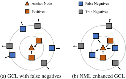
The prevailing approach in GCL aims to maximize mutual information (MI) between different views, bringing positive sample embeddings closer together while pushing negative sample embeddings further apart [Veliˇckovi´c et al., 2018; Zhu et al., 2020]. For this purpose, InfoNCE, a lower bound of MI, is widely applied as the contrastive loss [Poole et al., 2019]. InfoNCE-based approaches often treat different views of the same node as positives, while those of different nodes as negatives. Such arbitrary and overly simplistic strategy makes the existing methods suffer from false negatives, i.e., the positive samples incorrectly treated as negatives. For example, in Fig. 1a, the GCL with false negatives will result in that the embeddings of false negatives (blue squares) and true negatives (grey squares) are pushed away together from the anchor node (red triangle), which undermines the discriminative power of the learned embeddings, thereby reducing the performance on downstream tasks [Chuang et al., 2020].
∗Corresponding author
The existing methods usually address the issue of false negatives by weighting negative samples, which fall into two categories, hard-weight based [Zhang et al., 2022; Wang et al., 2024; Hu et al., 2021; Liu et al., 2023; Wu et al., 2020; Huynh et al., 2022; Fan et al., 2023; Han et al., 2023; Sun et al., 2023; Yang et al., 2022; Li et al., 2023; Liu et al., 2024] and soft-weight based [Xia et al., 2022; Lin et al., 2022; Hao et al., 2024; Liu et al., 2024; Niu et al., 2024; Zhuo et al., 2024b; Wan et al., 2023; Chi and Ma, 2024; Zhuo et al., 2024a]. In particular, hard-weight based methods often assign binary weights to negative samples based on predefined criteria such as similarity threshold [Wu et al., 2020; Huynh et al., 2022] or neighborhood distance [Li et al., 2023; Liu et al., 2024; Zhang et al., 2022]. For instance, in [Zhang et al., 2022], the first-order neighbors of an anchor node are considered false negatives. In contrast, soft-weight based methods relax the weight to [0, 1], of which one typical approach is first cluster the nodes, then determine the weight of negative samples based on the distance between the anchor node and the cluster where the negative sample resides [Lin et al., 2022]. However, both methods rely on simple prior knowledge to identify false negatives, which cannot guarantee precision or recall, still leading GCL to suboptimal results.
To overcome the above challenges, in this paper, we propose a novel Negative Metric Learning (NML) enhanced GCL (NML-GCL). The main idea of NML-GCL is to extend an InfoNCE-based GCL with a Negative Metric Network (NMN) to build a negative metric space where the less likely two nodes are true negatives of each other (and equivalently, the more likely two nodes are false negatives of each other), the closer their distance. As shown in Fig. 1b, compared with the true negatives, the false negatives' embeddings will be pulled closer to the anchor node under the guidance of the negative metric network. Essentially, this distance in the negative metric space can be considered a soft label indicating the node's status as a negative or positive sample with respect to the anchor. However, in the situation of self-supervised learning, the training of the negative metric network is difficult because there is a lack of explicit supervision signals regarding on negative/positive samples. To address this issue, inspired by the idea of self-training [Wei et al., 2020], we propose a joint training scheme that can iteratively update the graph encoder (GCN) and the negative metric network with a bi-level optimization objective. During the bi-level optimization, the negative metric network is responsible for assigning soft labels to samples based on the embeddings output by the encoder, while the encoder adjusts itself in the next iteration based on these soft labels. It is noteworthy that the insight here is the self-supervision signals (i.e., the different views of an anchor node) not only explicitly supervise the training of the encoder, but also implicitly supervise the training of the negative metric network, which makes them able to help each other.
We further provide a solid theoretical analysis of our proposed NML-GCL, revealing the connection between the negative metric network and the graph encoder. Specifically, we prove that: (1) our NML can enhance the GCL with a tighter lower bound of mutual information (MI) compared to traditional InfoNCE loss, and (2) by maximizing the tighter lower bound of MI, the joint training of the encoder and the negative metric network can mutually reinforce each other, leading to simultaneous improvements. Our contributions are summarized as follows:
- We propose a novel GCL framework NML-GCL. NMLGCL employs a learnable negative metric network to build a negative metric space, in which false negatives can be distinguished better from true negatives based on their distance to anchor node.
- To overcome the lack of explicit supervision signals for NML, we propose a joint training scheme with bi-level optimization objective, which implicitly utilizes the selfsupervision signals to iteratively optimize the encoder and the negative metric network.
- Furthermore, we provide a solid theoretical justification of NML-GCL, by proving that due to NML, NML-GCL can approximate the MI between contrastive views with
- a tighter lower bound than traditional InfoNCE loss, which leads to the superiority of NML-GCL to the existing GCL methods.
- The extensive experiments conducted on real-world datasets demonstrate the superiority of NML-GCL, in terms of the performance of the downstream tasks and the identifying of false negatives.
Due to space limitations, related work is presented in Appendix ??.
2 Preliminaries
A graph is denoted by G = (V, E), where V = {i}Ni=1 , E ⊆ V × V represent the set of N nodes and the set of edges respectively. Let A ∈ {0, 1}N×N denote the adjacency matrix and X ∈ RN×F be the node attribute matrix, where cell aij at i-th row and j-th column of A is 1 if (i, j) ∈ E, otherwise 0, xi ∈ RF is the i-th row of X representing the attribute vector of node i, and F is the dimensionality.
2.1 Graph Contrastive Learning
GCL follows an augmentation-encoding-contrasting mechanism basically. In the augmentation stage, GCL creates contrastive views preserving invariant structural information and feature information, by perturbing original graphs, e.g., edge masking [Rong et al., 2020; You et al., 2020], node feature perturbation [You et al., 2020], or graph diffusion [Hassani and Khasahmadi, 2020]. In the encoding stage, GCL employs a GCN as encoder to generate the node embeddings, which is usually defined as
where H(k) is the node embedding matrix at layer k, ˜A is the normalized adjacency matrix, andWk is the trainable weight matrix of layer k.
In the contrasting stage, the encoder is optimized by maximizing the agreement between the contrastive views, which is usually implemented with the InfoNCE loss [Poole et al., 2019] defined as:
where ui and vi are the embeddings of node i in contrastive views GU and GV , respectively, θ(·, ·) is a similarity function (e.g., cosine), τ is a temperature parameter.
2.2 False Negatives
Let Si be the negative sample set of an anchor node i generated by a sampling strategy. Then the false negatives of anchor node i with respect to Si can be defined as
Definition 1 (False Negatives). Node j is a false negative of anchor node i if j ∈ Si and Y (j) = Y (i), where Y (·) be the oracle label function unknown in advance.
The idea of the above definition is that a false negative j is a positive (Y (j) = Y (i)), but is treated as a negative (j ∈ Si), since the node labels are unobserved (i.e., Y (·) is unknown). In contrast, the true negatives are the nodes with labels different to the label of the anchor node.
3 Methodology
3.1 Overview
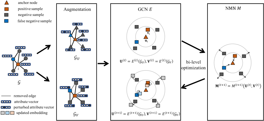
Fig. 2 presents an overview of our proposed NML-GCL. From Fig. 2 we can see that in the augmentation stage, NMLGCL first generates two contrastive views GU and GV , each of which perturbs both the graph topology and the attributes of nodes of the original graph G. And then, the two augmentations GU and GV are sent to the GCN encoder E defined in Equation (1) to obtain the two node embedding matrices U = E(GU) ∈ RN×d and V = E(GV ) ∈ RN×d for contrastive learning, where d is the embedding dimensionality. In the contrastive learning stage, for an anchor node i ∈ V, (ui, vi), which are i-th rows of U and V representing the embeddings of i in views GU and GV respectively, is selected as the positive pair, while {(ui, vj)}j∈V as the negative pairs. Note that here in our NML-GCL, (ui, vi) is considered as both positive and negative pair, so that their embedding distance can be adjusted by negative metric network (NMN) together with other negative pairs in a unified way.
NML-GCL employs a bi-level optimization to jointly train GCN E and negative metric network M in an iterative fashion. In (t + 1)-th iteration, NML-GCL first updates M to M (t+1) with respective to the contrastive node embeddings U(t) and V(t) ∈ RN×d generated by GCN E(t) in previous iteration. Then NML-GCL uses M (t+1) to obtain the new negative metric matrix M(t+1) ∈ RN×N . At last, GCN E is updated to E(t+1) with respective to M(t+1) . In the negative metric matrix M, the cell at i-th row and j-th column mij measures how likely node j is a negative of node i. As mentioned before, mij can be regarded as a soft label of j indicating its status as a negative sample with respective to the anchor node i.
3.2 Negative Metric Learning
To deal with the false negatives in GCL, we introduce Negative Metric Learning (NML) to learn a negative metric network M. The negative metric network M captures the distance between two nodes from different views in the negative metric space, which reflects the probability they are negatives of each other. In particular, M consists of an MLP and a normalizing layer, which is defined as
where m′ij is the distance between ui and vj in the negative sample space and mij ∈ [0, 1] is the normalized distance w.r.t. ui satisfying ∑j mij = 1. Therefore, mij can be regarded as the probability (soft label) that j is a negative of i.
We expect M outputs smaller mij for a false negative j of an anchor node i. As mentioned before, however, there are no explicit supervision signals telling us false negatives. To overcome this issue, we introduce the similarity θ(ui, vi) induced by the GCN E as the surrogate supervision signals for the training of M, by which the self-supervision signals (i.e., the supervision offered by the fact (ui, vi) is positive pair) are transferred to the training of M. θ can be any qualified similarity measures, e.g., cosine. Based on this idea, the optimization objective of M can be formulated as
where
is a contrastive loss of anchor node i with the temperature parameter τ. It is obvious that when minimizing L(i) NML w.r.t. M, the bigger θ(ui, vj), the smaller mij. Note that, compared with traditional InfoNCE loss defined by Equation (2) where each j ̸= i is treated as negatives of i with constant weight 1, in Equation (5) all nodes j ∈ V, even i itself, are treated as potential negatives of i, and the weight of a negative becomes a learnable metric mij induced by the negative metric network M.
To further clarify how the self-supervised signals implicitly supervise the training of M, we transform the loss defined by Equation (5) to an approximate hinge loss via the following derivation:
≈ max {x1, x2, ..., xn} [Zhang et al., 2024].
As we will demonstrate later, under the guidance of the self-supervised signal that (ui, vi) is positive pair, we can train a GCN E capable of generating node embeddings that satisfy θ(ui, vi) ≥ θ(ui, vj) for j ̸= i. Therefore, Equation (6) indicates that once E is trained, the minimization of L(i) NML w.r.t. M implicitly requires smaller mii due to the bigger θ(ui, vi), which leads to a higher probability, via smaller mii, to the event that vi is a false negative of ui. In other words, via bigger θ(ui, vi), the self-supervision signals can strengthen M's ability to recognize false negatives by enforcing a smaller mii.
3.3 Bi-level Optimization
We have seen that the training of M depends on a reliable θ(ui, vj) induced by E, and however, the training of E is guided by the negative metric matrix output by M. Our idea to break this dilemma is to iteratively optimize them with following bi-level optimization:
where L(i) reg is the regularization loss and α controls the weight of the regularization. L(i) reg is defined as
where KL(·||·) is KL-divergence, Pi is the distribution over {mij}j∈V given i, i.e., Pi(j) = mij, and P0 is a uniformly distribution, i.e., P0(j) = 1/N. L(i) reg constrains the feasible region of the i-th row mi of the negative metric matrix M to prevent mi from becoming a one-hot vector.
During the (t + 1)-th iteration of the bi-level optimization defined in Equation (7), the inner minimization will result in optimal M(t+1) , which is supervised by θ(U(t) ,V(t) ) induced by the node embeddings offered by E(t) , as described in Section 3.2. Now we want to answer two questions for the outer minimization.
(1) How does M(t+1) supervise the training of E(t+1) through L(i) NML ? Again according to Equation (6), the minimization of L(i) NML w.r.t. E requires to minimize max {0, θ(u(t+1) i , v(t+1) j ) - θ(u(t+1) i , v(t+1) i ) + log ((N - 1)m(t+1) ij )}. For this purpose, E has to be adjusted to make sure that θ(u(t+1) i , v(t+1) j ) is smaller than θ(u(t+1) i , v(t+1) i ) by at least log ((N - 1)m(t+1) ij ). Obviously, the bigger m(t+1) ij , the smaller θ(u(t+1) i , v(t+1) j ). In other words, here m(t+1) ij supervises the training of E(t+1) by telling it how far it should push v(t+1) j away from v(t+1) i .
(2) What is the relation between E(t+1) and E(t) ? As the training of E(t+1) is supervised by M(t+1) , to answer this question, we need to take a lose look at M(t+1) . Obviously, for an anchor node i ∈ V, the optimal m(t+1) ik (k ∈ V) satis-
and
which together lead to the optimal
From Equation (11), we can see that m(t+1) ik is inversely proportional to the similarity θ(u(t) i , v(t) k ). This means that if E(t) pushes vk from vi (i.e., smaller θ(u(t) i , v(t) k )), which leads to bigger m(t+1) ik , then E(t+1) will push vk even farther from vi under the supervision of m(t+1) ik (see the answer of Question (1)). This result shows that the training of E can be regarded as a form of self-training [Wei et al., 2020], where the supervision signal is provided by E via M.
Finally, the above analysis also shows that due to the iterative updating, the negative metric network M, which captures the distance in negative metric space, and the encoder E, which generates discriminative embeddings, would reinforce each other during the bi-level optimization. As we will theoretically justify in the later, the bi-level optimization accurately maximizes the mutual information between contrastive views, which leads to E and M capable of distinguishing false negatives from true negatives. The complete training process is presented in Algorithm 1, and its time complexity analysis is shown in Appendix ??.
Algorithm 1 Training process of our proposed NML-GCL
Input: A graph G, an encoder E, a negative metric network M, the number of training epochs TE for outer minimization, the number of iterations TM for inner minimization; Output: The optimal encoder E;
- 1: Initialize parameters of E andM;
- 2: for i = 1, 2, · · · , TE do
- 3: Randomly generate contrastive views GU and GV from G;
- 4: Generate node embeddings U and V by E;
- 5: // Training negative metric network
- 6: Freeze parameters of E;
- 7: for j = 1, 2, · · · , TM do
- 8: Update M according to Equation (7);
- 9: end for
- 10: // Training Encoder
- 11: Freeze parameters of M;
- 12: Update E according to Equation (7);
- 13: end for
4 Theoretical Analysis
In this section, we first prove that compared with traditional InfoNCE-based GCL, our NML-GCL maximizes a tighter lower bound of the mutual information (MI) between contrastive views. Then we demonstrate that the maximization of the MI endows the encoder E and the negative metric network M with the ability to distinguish false negatives from true negatives.
4.1 Tighter Lower Bound of MI
Let U and V be random variables representing node embeddings in contrastive views GU and GV , respectively, and I(U; V ) be their MI. Let INML(U; V ) and INCE(U; V ) denote the MI estimated by L(i) NML defined in Equation (5) and traditional InfoNCE loss LInfoNCE defined in Equation (2), respectively. The following theorem shows that INML(U; V ) is a tighter lower bound of I(U; V ) than INCE(U; V ).
Theorem 1. I(U; V ) ≥ INML(U; V ) ≥ INCE(U; V ), where INML (U; V ) = -minM Ei∈V[L(i) NML ] + C, INCE(U; V ) = LInfoNCE + C and C = log N.
The detailed proof of Theorem 1 can be seen in Appendix ??. Basically, Theorem 1 offers the rationality of NMLGCL's bi-level optimization by which NML-GCL achieves better generalizability on downstream tasks than traditional InfoNCE based GCL methods.
4.2 MI Maximization Facilitates NML
Theorem 1 shows that the minimization of L(i) NML in each iteration of the bi-level optimization defined in Equation (7) approximately maximizes I(U; V ) by maximizing its tighter lower bound INML(U; V ). Now we further demonstrate that the maximization of I(U; V ) facilitates NML, enabling the encoder and the negative metric network to ultimately acquire the ability to distinguish between false negatives and true negatives in the negative metric space learned by NML. At first, the following theorem shows that an optimal E can simulate the oracle label function Y by appropriately ranking the distance of samples to a given anchor node in the negative metric space.
Theorem 2. If E∗ =maxE EGU,GV I(U; V ), then
where d(·, ·) is a distance metric, S - i is the true negative set of i, S + i is the false negative set of i, and zi represents the embedding of node i in original graph G generated by encoder E∗ .
The proof of Theorem 2 can be found in Appendix ??. Theorem 2 tells us that after maximizing I(U; V ), in the embedding space defined by E∗ , the expected distance from false negatives to an anchor node is shorter than the expected distance from true negatives to the anchor node. In other words, E∗ can simulate the behavior of the oracle label function Y , since d(zi, zj) approaches to 0 if Y (j) = Y (i), which explains why our NML-GCL is able to obtain node embeddings that are more discriminative in terms of class distinction.
Theorem 2 together with Theorem 1 and Equation (11) justifies that E and M can iteratively reinforce each other via the bi-level optimization. Specifically, in one iteration, the inner minimization results in better M that offers better supervision for the training of E; the outer minimization results in better E that can induce more reliable {θ(ui, vj)} as the supervision for the training of M in next iteration. Such positive feedback loop ensures the effectiveness of our NML-GCL.
5 Experiments
In this section, we conduct experiments to answer the following research questions (RQs):
- RQ1: Does NML-GCL outperform existing GCL methods on downstream tasks?
- RQ2: How Negative Metric Network M contributes to the performance of NML-GCL?
- RQ3: How do the hyper-parameters affect the performance of NML-GCL?
We conduct additional experiments, including experimental verification of theoretical analysis and the identification of false negatives, as detailed in Appendix ??.
5.1 Experiment Settings
Datasets. We conduct experiments on six publicly available and widely used benchmark datasets, including three citation networks Cora, CiteSeer, PubMed [Yang et al., 2016], two Amazon co-purchase networks (Photo, Computers) [Shchur et al., 2018], and one Wikipedia-based network Wiki-CS [Mernyei and Cangea, 2020]. The statistics of datasets are summarized in Table ?? in Appendix ??.
| Method | Cora | CiteSeer | PubMed | Photo | Computers | Wiki-CS |
|---|---|---|---|---|---|---|
| BGRL | 82.22±0.51 | 72.27±0.26 | 79.41±0.23 | 93.01±0.27 | 88.25±0.30 | 77.81±0.42 |
| GRACE | 81.52±0.24 | 70.12±0.17 | 78.32±0.45 | 91.88±0.18 | 87.15±0.21 | 77.95±0.23 |
| MVGRL | 81.15±0.16 | 70.46±0.23 | 78.63±0.27 | 92.59±0.34 | 87.66±0.25 | 78.52±0.15 |
| LOCAL-GCL | 83.86±0.21 | 71.78±0.48 | 80.95±0.41 | 92.83±0.28 | 88.69±0.50 | 78.98±0.52 |
| PHASES | 82.19±0.37 | 70.49±0.40 | 81.08±0.62 | 92.74±0.37 | 87.80±0.44 | 79.61±0.29 |
| HomoGCL | 83.19±1.03 | 70.11±0.79 | 81.02±0.68 | 92.31±0.36 | 87.82±0.48 | 78.18±0.45 |
| GRACE+ | 82.84±0.18 | 70.57±0.53 | 81.13±0.31 | 92.73±0.35 | 88.56±0.31 | 79.33±0.27 |
| ProGCL | 82.04±0.27 | 70.63±0.22 | 78.14±0.43 | 92.71±0.29 | 87.90±0.27 | 78.21±0.41 |
| GRAPE | 83.88±0.04 | 72.34±0.22 | OOM | 92.76±0.30 | 87.97±0.33 | 79.91±0.16 |
| NML-GCL | 84.93±0.14 | 73.37±0.13 | 82.10±0.30 | 93.36±0.21 | 89.43±0.25 | 80.32±0.18 |
| (p-value) | (9.88e-15) | (1.89e-10) | (1.25e-6) | (4.58e-3) | (5.55e-4) | (4.07e-5) |
| w/o M | 82.82±0.07 | 70.31±0.17 | 80.14 ±0.14 | 92.12 ±0.16 | 87.76 ±0.19 | 77.91 ±0.24 |
| repl. cosine sim. | 83.87±0.22 | 71.18 ±0.24 | 81.31 ±0.24 | 92.80 ±0.22 | 88.35 ±0.21 | 79.13 ±0.14 |
Baselines. To validate the effectiveness of our NML-GCL, we compare it with state-of-the-art GCL methods including:
- three methods without considering false negatives, BGRL [Thakoor et al., 2021], GRACE [Zhu et al., 2020], and MVGRL [Hassani and Khasahmadi, 2020],
- three methods dealing with false negatives with hard weight, LOCAL-GCL [Zhang et al., 2022], PHASES [Sun et al., 2023], HomoGCL [Li et al., 2023],
- three methods dealing with false negatives with soft weight, GRACE+ [Chi and Ma, 2024], ProGCL [Xia et al., 2022], and GRAPE [Hao et al., 2024], where ProGCL and GRAPE determine the weights based on clustering.
Evaluation Protocols. We follow a two-stage evaluation protocol widely used by existing works [Zhang et al., 2021; Zhu et al., 2020]. For each method, in the first stage, we generate node embeddings, while in the second stage, we evaluate the node embeddings in terms of the performance of node classification and node clustering. Specifically, for node classification, the classifier is implemented as a logistic regression. The node embeddings generated by a baseline method or NML-GCL is split into a training set, a validation set, and a testing set. The training set and validation set are used for the training and hyper-parameter tuning of the classifier, while testing set for evaluation in terms of accuracy. For node clustering, we use k-means algorithm to partition the node embeddings where k is set to the number of classes in a dataset, and evaluate the clustering results by two widely used metrics, Fowlkes-Mallows Index (FMI) [Campello, 2007] and Adjusted Rand Index (ARI) [Steinley, 2004].
Configurations. In NML-GCL, the encoder E is implemented as a two-layer GCN with embedding dimensionality d = 512, and the NMN is implemented as an MLP with two hidden layers each of which consists 512 neurons. We apply Adam optimizer for all the GCL methods and the classifier. Following the approach of [Zhu et al., 2020], we adopt DropEdge [Rong et al., 2020] and FeatureMasking [You et al., 2020] to generate contrastive views. The detailed hyperparameter settings are shown in Table ?? in Appendix ??.
5.2 Performance on DownstreamTasks (RQ1)
Results of Node Classification. To train the classifier, we follow the public splits on Cora, CiteSeer, and PubMed, and a 1:1:8 training/validation/testing splits on the other datasets. The reported results are averaged over 10 runs with random seeds, and the average classification accuracies with standard deviation are reported in Table 1. We see that NMLGCL consistently outperforms all the baseline methods, especially the soft-weight based ones (GRACE+, ProGCL, and GRAPE) and the hard-weight based ones (LOCAL-GCL, PHASES, and HomoGCL). Moreover, we conduct the paired t-test on NML-GCL and the best baseline. The p-value in the third-to-last line shows that all the p-values are smaller than 0.01, indicating that the improvement achieved by NMLGCL is statistically significant. This improvement is because via the bi-level optimization, NML learns a negative metric space where false negatives are closer to anchor than true negatives. Due to NML, NML-GCL is able to suppress the impact of false negatives according to the learned distance to anchor nodes, which makes the optimization orientation of the encoder be rectified towards better distinguishing false negatives from true negatives, resulting in node embeddings with stronger discriminability. In addition, methods addressing false negatives are generally superior to those that do not consider them, highlighting that suppressing the disturbance of false negatives enhances GCL's ability to generate more robust and generalizable node embeddings.
Results of Node Clustering. Table 2 shows FMI and ARI of clustering conducted with k-means algorithm over the node embeddings generated by baseline methods and NMLGCL. At first, NML-GCL consistently outperforms the baseline methods in terms of both metrics, indicating that the clustering based on NML-GCL can result in purer clusters, i.e., a cluster contains only nodes of the same label, and the nodes of the same class are grouped into the same cluster.
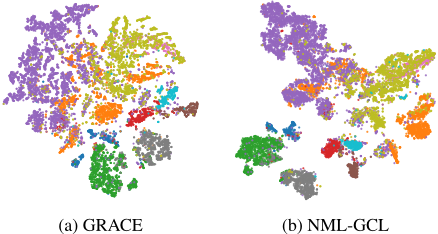
As a study, we visualize the clustering results of NMLGCL and GRACE on the Computers dataset by t-SNE in Figs. 3a and 3b, respectively. We can see that compared with the traditional InfoNCE based method GRACE, NML-GCL can produce clustering results with higher intra-cluster cohesion and clearer inter-cluster boundaries. This is because NMLGCL, aided by negative metric learning, brings positive examples (including false negatives) closer together and pushes positive and true negative examples farther apart more effectively.
| Method | Cora | CiteSeer | PubMed | Photo | Computers | Wiki-CS | ||||||
|---|---|---|---|---|---|---|---|---|---|---|---|---|
| FMI | ARI | FMI | ARI | FMI | ARI | FMI | ARI | FMI | ARI | FMI | ARI | |
| BGRL | 52.74 | 42.82 | 46.37 | 34.27 | 54.40 | 28.44 | 62.59 | 50.34 | 45.37 | 31.68 | 36.16 | 27.96 |
| GRACE | 53.24 | 43.68 | 45.36 | 33.71 | 51.47 | 24.63 | 57.27 | 47.42 | 46.83 | 35.22 | 37.61 | 28.24 |
| MVGRL | 55.49 | 46.68 | 47.43 | 37.82 | 51.52 | 24.97 | 57.67 | 48.04 | 45.74 | 33.75 | 35.16 | 25.53 |
| LOCAL-GCL | 51.33 | 40.53 | 47.98 | 36.34 | 54.08 | 27.15 | 61.78 | 48.02 | 46.15 | 33.16 | 38.25 | 29.14 |
| PHASES | 53.77 | 44.22 | 49.38 | 38.50 | 50.88 | 23.35 | 56.45 | 48.51 | 45.71 | 35.97 | 40.43 | 30.74 |
| HomoGCL | 56.71 | 47.13 | 49.06 | 38.28 | 58.05 | 33.54 | 62.37 | 53.26 | 48.50 | 37.14 | 40.25 | 31.33 |
| GRACE+ | 55.36 | 45.92 | 49.91 | 39.62 | 54.20 | 28.36 | 61.88 | 53.94 | 48.08 | 36.66 | 43.59 | 35.02 |
| ProGCL | 56.00 | 46.52 | 49.90 | 38.98 | 52.14 | 25.60 | 62.14 | 50.32 | 48.27 | 36.44 | 39.12 | 29.21 |
| GRAPE | 56.50 | 47.45 | 50.87 | 40.39 | OOM | OOM | 62.24 | 53.73 | 48.84 | 38.67 | 40.85 | 32.03 |
| NML-GCL | 58.23 | 49.50 | 52.46 | 42.19 | 59.81 | 35.82 | 63.13 | 55.56 | 50.52 | 39.42 | 45.46 | 37.74 |
5.3 Ablation Study (RQ2)
In this section, we demonstrate the necessity of NMN M in NML-GCL. Specifically, we compare NML-GCL with the following variants: (1) w/o M: We remove the negative metric network, and mij is a constant (i.e., 1N ); (2) repl. cosine sim.: mij is calculated as exp(-cosine similarity(ui, vi)).
As shown in the last two rows of Table 1, we see the NMN component contributes to the performance improvement of NML-GCL, especially with a 3% gain on CiteSeer. Moreover, although the use of cosine similarity can alleviate the problem of false negatives to some extent, NML-GCL uses the NMN M to capture the nonlinearity in the distance measurement, so that false negatives can be better distinguish from true negatives in the negative metric space. Overall, the results highlight that the inclusion of M in NML-GCL is essential for refining the negative sample learning process, enabling a more nuanced and effective representation of negative pairwise distances. This demonstrates the critical role of NMN in achieving superior performance compared to simpler, predefined negative sample weighting strategies like cosine similarity.
5.4 Hyper-parameter Analysis (RQ3)
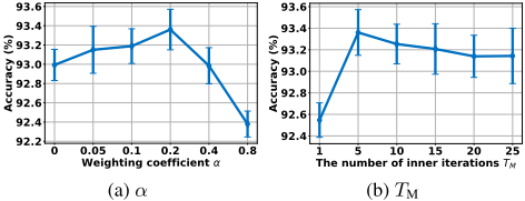
Now we investigate the effectiveness of the two most important hyper-parameters α in Equation (7) and the iteration number TM of inner minimization in Algorithm 1. We take the Photo dataset as an example. Fig. 4a shows that as α increases, the classification accuracy first rises and then falls. Since α is the weight of the regularization term in Equation (7), this result indicates that when α is small, NML-GCL suffers from overfitting. In contrast, when α becomes large, the weight distribution of negatives tends to become uniform, causing the learned embeddings to lose their discriminability. From Fig. 4b, we see that too few iterations of the inner minimization can lead to underfitting, while too many iterations can cause overfitting and unnecessary wasting of time.
6 Conclusion
In this paper, we introduce a novel approach called NMLGCL. NML-GCL utilizes a learnable negative metric network to construct a negative metric space, allowing for better differentiation between false negatives and true negatives based on their distances to the anchor node. To address the challenge of the lack of explicit supervision signals for NML, we present a joint training scheme with a bi-level optimization objective that implicitly leverages self-supervision signals to iteratively refine both the encoder and the negative metric network. Comprehensive theoretical analysis and extensive experiments conducted on widely used benchmarks demonstrate the superiority of our proposed method to baseline methods on downstream tasks.
Contribution Statement
Yiyang Zhao, Chengpei Wu, and Lilin Zhang made equal contribution to this work and share the first authoship.
Acknowledgements
This work is supported by Natural Science Foundation of Sichuan Province under grant 2024NSFSC0516 and National Natural Science Foundation of China under grant 61972270.
@inproceedings{ijcai2025p794,
  title     = {Negative Metric Learning for Graphs},
  author    = {Zhao, Yiyang and Wu, Chengpei and Zhang, Lilin and Yang, Ning},
  booktitle = {Proceedings of the Thirty-Fourth International Joint Conference on
               Artificial Intelligence, {IJCAI-25}},
  publisher = {International Joint Conferences on Artificial Intelligence Organization},
  editor    = {James Kwok},
  pages     = {7137--7145},
  year      = {2025},
  month     = {8},
  note      = {Main Track},
  doi       = {10.24963/ijcai.2025/794},
  url       = {https://doi.org/10.24963/ijcai.2025/794},
}
TY - CPAPER TI - Negative Metric Learning for Graphs AU - Zhao, Yiyang AU - Wu, Chengpei AU - Zhang, Lilin AU - Yang, Ning T2 - Proceedings of the Thirty-Fourth International Joint Conference on Artificial Intelligence, IJCAI-25 PB - International Joint Conferences on Artificial Intelligence Organization PY - 2025 SP - 7137 EP - 7145 DO - 10.24963/ijcai.2025/794 UR - https://doi.org/10.24963/ijcai.2025/794 ER -Copied
Machine-readable versions of this paper, for tools and AI agents:





