What Makes You Special? Contrastive Heuristics Based on Qualified Dominance

1 Introduction

The most common approach for cost-optimal planning is to use A∗ [Hart et al., 1968] with a heuristic function that estimates the goal distance from each state. To ensure optimality the heuristic should be admissible, meaning that the real distance is never overestimated. However, the search effort can grow exponentially with almost perfect heuristics, even for problems solvable in polynomial time [Pearl, 1984; Helmert and R¨oger, 2008]. This naturally raises the question of how to extend the notion of heuristics to gain more expressive power.

We introduce contrastive heuristics, which estimate goal distance by considering previously explored nodes. Similar ideas appear in novelty heuristics [Katz et al., 2017; Lipovetzky and Geffner, 2017; Groß et al., 2020; Singh et al., 2021; Rosa and Lipovetzky, 2024], which use state statistics to diversify search but lack formalization of the search and lose optimality guarantees. In [Karpas and Domshlak, 2012] they propose an inadmissible heuristic that retains optimality by considering alternative paths. Contrastive heuristics provide a formal framework for search-state-dependent heuristics that retain optimality while relaxing admissibility. We prove that A∗ with contrastive heuristics remains optimal if for each inadmissible node there is a better node that is admissible. Thus, goal distance can be evaluated in contrast to other nodes, i.e. through paths only available to this node.

We also show how to automatically construct contrastively admissible heuristics for any planning task. To this end, we extend dominance pruning, which prunes states s shown to be at least as far from the goal as some t [Torralba and Hoffmann, 2015]. But full dominance is often hard to guarantee. Thus, our second contribution is qualified dominance. When t does not dominate s, we ask: "Why? What can s do that t cannot?" We characterize this as a set of plans from s for which no equivalent from t could be proven. We show how to automatically synthesize a finite-state automaton whose language captures plans from s that are dominated by t.

Finally, we show that qualified dominance information can be encoded in the description of the planning task, so any domain-independent admissible heuristic that can estimate the goal-distance for any planning task can be used to compute contrastive heuristic estimates. We provide a first implementation on top of the operator-counting framework [Pommerening et al., 2014]. Our experiments show that our qualified dominance techniques are able to find information across many tasks, even though this is not very complementary with highly informative heuristics.

2 Background

A labelled transition system (LTS) is a tuple Θ = (S, L, T, SI , SG), where S is a set of states, L is a set of labels with cost c(ℓ) ∈ R+, 1 , T ⊆ S×L×S is a transition relation, and SI , SG ⊆ S are the set of initial and goal states, respectively. Typically, there is a single initial state. However, considering a set of initial states simplifies the notation [B¨uchner et al., 2024]. We write s ℓ-→Θ s′ whenever (s, ℓ, s′ ) ∈ T, or simply s ℓ-→ s′ if the Θ is clear from context.

A path from s0 to sn in Θ is a sequence of transitions s0 ℓ1 -→ s1 . . . ℓn -→ sn. L∗ is the set of finite sequences of labels and ε is the empty sequence. A plan π ∈ L∗ for a state s ∈ S is a sequence of labels s.t. there exists a path from s to sn ∈ SG. The cost of π is c(π) = ∑ℓ∈π c(ℓ). We denote by P(s) the set of all plans from s to a goal state, or by PΘ(s)

1 We assume non-zero cost labels to simplify the notation. But we can support 0-cost labels by treating them as having ϵ-cost.

for a particular LTS Θ. We denote h∗ (s) = minπ∈P (s) c(π′ ). A plan for s is optimal if c(π) = h∗ (s). We look for a plan from s0 ∈ SI with cost h∗ (SI ) = mins0∈SI h∗ (s0).

We consider planning tasks in factored transition system (FTS) representation [Sievers and Helmert, 2021; Torralba and Sievers, 2019; B¨uchner et al., 2024]. An FTS task T = (Θ1, . . . ,Θn) is a tuple of LTSs, called factors, with a common set of labels, such that Θi = (Si, L, Ti, SI i , SG i ). We use a tuple, instead of a set, to refer to the individual factors by their index. We denote by ◦ tuple concatenation. States in the individual factors si ∈ Si are called facts. A state in T is a tuple of facts s = (s1, . . . , sn), one for each factor, si ∈ Θi.

The FTS task compactly describes the state space. This is another LTS ΘT = Θi ⊗ . . . ⊗ Θn = (ST , L, TT , SIT , SG T ), where ST = S1 × · · · × Sn is the Cartesian product of each factor's states, TT = {((s1, . . . , sn), ℓ, (t1, . . . , tn) | (si, ℓ, ti) ∈ Ti for 1 ≤ i ≤ n}, SIT = SI 1 × · · · × S In , and SG T = SG 1 × · · · × SG n . Note that the order of the factors is fixed, but arbitrary, as the resulting products for different orderings are isomorphic. Throughout the paper, we use subscripts to differentiate states in ST (e.g., s, s′ , t) and facts from each factor Θi (e.g., si, s′i , ti) so that si = s[i].

An LTS is deterministic if (s, ℓ, s′ ), (s, ℓ, s′′ ) ∈ T implies s′ = s′′ , and |SI | = 1. An FTS task T is deterministic if all of its factors are deterministic, which implies that the state space ΘT is also deterministic. Tasks in other common planning formalisms such as STRIPS [Fikes and Nilsson, 1971] and SAS+ [B¨ackstr ¨om and Nebel, 1995] can be compiled into a deterministic FTS task [Sievers and Helmert, 2021].

A heuristic is a function hT : S → R+0 that estimates the cost of the cheapest path from a state to a goal state in a planning task T . The planning task is omitted when it is clear from context. A heuristic is admissible if it never overestimates the cost, i.e. h(s) ≤ h∗ (s) for all s ∈ S.

The most common algorithm for optimal planning is A∗ [Hart et al., 1968]. A search node ns represents a path from the initial state to the state s, and g(ns) denotes the cost of the path. We denote by N the set of all search nodes for a state space. A∗ maintains a closed and an open list of all the search nodes seen so far. The open list is initialized with a node for each s0 ∈ SI , representing the empty path from s0. A node is expanded by removing it from the open list, adding it to the closed list, and adding all of its successors to the open list. A∗ iteratively expands a node with minimal f -value until a goal state is reached, where f(ns) = g(ns) + h(s). When h is admissible, A∗ is guaranteed to find the optimal plan. We also define f ∗ (ns) = g(ns) + h∗ (s).

A dominance relation is a relation ⊑ ⊆ S × S, s.t. s ⊑ t =⇒ h∗ (t) ≤ h∗ (s) [Torralba and Hoffmann, 2015]. Intuitively, s ⊑ t means that t is at least as close to the goal as s. In dominance pruning, a node ns can be pruned whenever there exists a node nt in the open or closed list s.t. s ⊑ t and g(nt) ≤ g(ns), thus guaranteeing that there is a plan through nt that is no more expensive than any plan through ns. A∗ with dominance pruning (A∗pr ) always finds an optimal plan.

To find dominance relations, we draw on the concept of simulation relations [Milner, 1971]. Specifically, a relation ⊑ is a cost-simulation for Θ if s ⊑ t implies that (i) t ∈ SG ∨s ̸∈ SG and (ii) ∀s ℓ-→ s′ ▪ ∃t ℓ′ -→ t′ ▪ c(ℓ′ ) ≤ c(ℓ) ∧ s′ ⊑ t′ . We always consider a noop transformation, adding a 0-cost label noop with a transition s noop ---→ s for all s ∈ S. This allows to reply to any transition s ℓ-→ s′ with t noop ---→ t whenever s′ ⊑ t. Any cost-simulation on ΘT is a dominance relation. This can be computed in polynomial time in the size of ΘT , but this is still exponential in the size of the planning task T .

To address this, one can compute a fact-dominance relation for each factor. For each Θi, we define a relation ⊑i⊆ Si×Si that allows us to express that a fact is as good as another. We also construct a label-relation ⪯i = {(ℓ, ℓ′ ) | ∀si ℓ-→Θi s′i ▪ ∃si ℓ′ -→Θi t′i ▪ s′i ⊑i t′i ∧ c(ℓ′ ) ≤ c(ℓ)} expressing that, on factor Θi, any time that ℓ can be applied, one can apply ℓ′ instead. Based on this, we can reason which labels can be applied without negative side effects on any other factor, ⪯¯i = ⋂j̸=i ⪯j . Finally, the label-dominance simulation technique computes a tuple (⊑1, . . . ,⊑n) of relations for each factor such that whenever si ⊑i ti then ti ∈ SG i ∨ si¬ ∈ SG i and ∀si ℓ-→ s′i ▪ ∃ti ℓ′ -→ t′i ▪ s′i ⊑i t′i ∧ ℓ ⪯¯i ℓ′ . Despite being a very recursive definition, the coarsest label-dominance simulation (⊑LD 1 , . . . ,⊑LD n ) can be computed in polynomial time in the size of the planning task [Torralba and Hoffmann, 2015]. Furthermore, one can compute a dominance relation for ΘT as s ⊑LD t iff si ⊑LD i ti for all i ∈ {1, . . . , n}.

Figure 1 shows the planning task of our running example, where a truck with limited amount of fuel delivers a package. It consists of 3 factors, representing the location of the truck, the package, and the amount of fuel. The initial state is (TA, PB, F2) and the goal states are of the form (·, PA, ·). Here, label-dominance simulation discovers that having more fuel is always better (F0 ⊑ F1 ⊑ F2). We also consider scaled versions of the task, e.g., with more fuel available.

3 Contrastive Heuristics

We generalize the notion of heuristics to contrastive heuristics, which evaluate states in the context of the search tree explored so far. Unlike traditional heuristics that estimate the cost to a goal independently for each state, a contrastive heuristic considers the relationship between states. In our running example (with many more than three fuel levels), suppose we have two states, s = (TA, PB, F70) and t = (TA, PB, F50), which are identical except that s has more fuel than t. If t has an optimal plan with cost 4, then this plan is also optimal for s, so the optimal heuristic value for both, when evaluated independently, is 4. However, when evaluating s in contrast to t, the heuristic value for s should be larger. This is because any plan for s that uses no more fuel than the plan for t could also be applied to t. If a drive action that consumes 1 fuel has cost 1, then the heuristic value of s in contrast to t should be at least 51. Any plan for s that uses less than 51 drive actions would also be valid for t. Thus, in this sense, the contrastive heuristic for s relative to t exceeds the independent heuristic value. Importantly, this heuristic is inadmissible since t has a plan, s has the same plan and thus the same goal distance. However, as we will show, this inadmissibility does not compromise optimality.

In this section, we formally define contrastive heuristics and demonstrate how they can be used in A∗ search to obtain optimal solutions.

Definition 1. A contrastive heuristic is a function η : N × 2N →R+0 , s.t. η(n,N) defines the heuristic value of node n in contrast to the nodes in N.

In contrast to a normal heuristic, a contrastive heuristic is defined for search nodes, and not states. This allows for even more information to be considered for heuristic evaluation, as the path to the node can also be taken into account, i.e. when considering N = ∅ it reduces to path-dependent heuristics [Bagchi and Mahanti, 1983; Richter et al., 2008; Karpas and Domshlak, 2009]. We call N the contrastive set.

Usually, admissibility of a heuristic is used to guarantee optimality of the search algorithm. However, in order to ensure the optimality of A∗ , it suffices that the heuristic always assigns an admissible value to at least one optimal node in the open list. We will consider a stricter requirement that is easier to reason about.

Definition 2. A contrastive heuristic η is contrastively admissible if for all ns, η(ns,N) ≤ h∗ (s) or there exists nt ∈ N s.t. η(nt,N) ≤ h∗ (t) ∧ f ∗ (nt) ≤ f ∗ (ns) ∧ (f ∗ (nt) < f ∗ (ns) ∨ h∗ (t) ≤ h∗ (s)).

Intuitively, a contrastively admissible heuristic guarantees that a node is assigned an inadmissible value only if there is a better node with an admissible value estimate. The contrapositive is that if there is no better node, then the node has an admissible value. Here, better means it has a lower f ∗ -value, or it has the same f ∗ -value but it is closer to the goal. The latter condition ensures for an optimal node in the open list, any better node must be in the open list as well.

Lemma 1. Let η be a contrastively admissible heuristic, and N ⊆ N a non-empty set of nodes, Nf ∗ = arg minn∈N f ∗ (n) and N ∗ = argminns∈Nf∗ h∗ (s). There exists a node ns ∈ N ∗ s.t. η(ns,N) ≤ h∗ (s).

Proof. Let ns ∈ N ∗ . From Definition 2, if η(ns,N) > h∗ (s), then there exists another node nt in N, that by construction is in N ∗ , such that η(nt,N) ≤ h∗ (t).

In order to utilize contrastive heuristics in A∗ search, we make a small modification to the search algorithm. Instead of expanding a node with minimum f-value, we expand the node with minimal ˆ f-value, given by ˆ fN(n) = g(n) + η(n,N). We denote by ˆ foc (n) = g(n) + η(n, open ∪ closed) the ˆ f-value that uses the union of the open and closed list as the contrastive set. We denote this version of A∗ as A∗oc .

Theorem 2. Let η be a contrastively admissible contrastive heuristic. A∗oc guarantees an optimal solution.

Proof. The proof is a modification of the proof of the optimality of A∗ from [Pearl, 1984, p. 78]. The optimal solution cost is f ∗ (ns0 ). We first show that there is always a node nt ∈ open s.t. ˆ foc(nt) ≤ f ∗ (nt) = f ∗ (ns0 ). By Lemma 1, there is a node nt with minimum f ∗ -value and minimum h∗ -value that is admissible. This node must be in open, otherwise its children would be in open and have smaller h∗ -value. Now, suppose A∗oc expands a goal node ns. We know that it's ˆ foc-value is minimal among all nodes in open. Therefore, ˆ foc(ns) ≤ f ∗ (nt), and ns is optimal.

The theorem above even holds when using a subset of open∪closed, because for a contrastive heuristic, if there is no better node in the contrastive set, then it must be admissible.

In practice, requiring the ˆ f-value of each node in the open list to be dependent on the current open and closed list is infeasible, as it requires recomputing the heuristic value for all nodes in the open list whenever a node is expanded. Instead, we evaluate each node upon generation, and keep the value fixed afterwards, resulting in different contrastive sets for each node. The algorithm is still optimal, as long as the heuristic cannot decrease when evaluated in a larger context.

Definition 3. A contrastive heuristic η is monotonic if for all n ∈ N and N,N ′ ⊆N N ⊆ N ′ =⇒ η(n,N) ≤ η(n,N ′ ).

The monotonicity property of the heuristic ensures that the ˆ f-value of a node will not decrease when increasing the contrastive set. This restriction is quite sensible, as it means that the heuristic value does not decrease when considering more information.

Theorem 3. Let η be a contrastively admissible monotonic heuristic and ν : N × 2N → 2N be any mapping s.t. ν(n,N) ⊆ N. A∗ with ˆ fν(n) = g(n) + η(n, ν(n, open ∪ closed)) guarantees an optimal solution.

Proof. From the monotonicity property, η(n, ν(n, open ∪ closed)) ≤ η(n, open ∪ closed) and thus ˆ fν(n) ≤ ˆ foc (n). Thus, we can consider ˆ fν to be an under-approximation of ˆ foc. With this, the same proof as of Theorem 2 is applicable.

4 Qualified Dominance

A dominance relation provides information about whether one state is at least as good as another. However, previous work only considers when a state is completely dominated and can be entirely removed from the search. Let us revisit the running example. The reason we could assign the state s = (TA, PB, F70) a higher heuristic value in contrast to t = (TA, PB, F50), is that we knew that if s does not use the additional fuel, t is just as good as s. This is a form of partial-dominance relation, where t dominates all plans of s that do not use more fuel than t has. In this section, we extend the notion of dominance to include some middle ground: the label sequences under which a state is dominated by another state. In this sense, we cannot completely prune the state, but we can disconsider these label sequences that can be simulated by the other state when computing heuristics.

Definition 4. A qualified dominance function is a function D : S×S → 2L∗ from a pair of states to a language over the labels, s.t. ∀π ∈ D(s, t) ▪ π ∈ P(s) =⇒ h∗ (t) ≤ c(π).

A qualified dominance function describes a subset of splans where t is guaranteed to have a no more expensive plan. Additionally, any label sequence that is not a plan of s is trivially dominated by t. Observe that a qualified dominance function does not need to be maximal, so the set of dominated plans can be arbitrarily underapproximated.

Qualified dominance generalizes the previous notion of a dominance relation, where t dominates s only if h∗ (t) ≤ h∗ (s). For any dominance relation ⊑, we can construct a qualified dominance function D⊑(s, t) = L∗ if s ⊑ t and D⊑(s, t) = ∅ otherwise. D⊑ and ⊑ are equivalent as D(s, t) = L∗ means that all splans are dominated by t. But qualified dominance can also express that certain paths are dominated even when a state is not fully dominated. In our running example, we can assign D((TA, PB, F70), (TA, PB, F50)) = { π ∈ L∗ | π has less than 51 drive actions }.

4.1 Inference of Qualified Dominance

Next, we consider how to represent and compute a qualified dominance function. We begin by describing how it can be defined over the entire state space of the planning taskthough this offers little practical value, as it is as hard as solving the task itself. We then show how it can be approximated by computing it over the factored task instead.

Definition 5. A function D : S × S → 2L∗ is a qualified ⪯-simulation for Θ if for all s, t ∈ S (i) ε ∈ D(s, t) only if t ∈ SG ∨ s ̸∈ SG and (ii) ℓ1ℓ2 . . . ℓn ∈ D(s, t) only if

Intuitively, a ⪯-simulation allows only to simulate a label with another label according to the label relation ⪯. An important special case is ℓ ⪯c ℓ′ iff c(ℓ′ ) ≤ c(ℓ) which we call a qualified cost-simulation.

Theorem 4. A qualified cost-simulation function is a qualified dominance function.

Proof. Let D be a cost-simulation function and π ∈ D(s, t). We show that either π ̸∈ P(s) or h∗ (t) ≤ c(π) by induction on the length of π. Base case (|π| = 0): from (i) of Definition 5, if s is not a goal, then π = ε ̸∈ P(s). If s and t are goals, then h∗ (t) = 0 = c(π). Induction step: Assume that the induction hypothesis holds for all |π′ | = n. Let π = ℓ1ℓ2 . . . ℓn+1. By (ii) of Definition 5, if s ℓ1 -→ s′ then there is t ℓ′1 -→ t′ s.t. c(ℓ′1 ) ≤ c(ℓ1) and ℓ2 . . . ℓn+1 ∈ D(s′ , t′ ). By the induction hypothesis, h∗ (t′ ) ≤ c(ℓ2 . . . ℓn+1), and thus h∗ (t) ≤ c(ℓ′1 ) + h∗ (t′ ) ≤ c(ℓ1ℓ2 . . . ℓn+1).

A qualified cost-simulation is a type of qualified dominance function. It enforces a simpler version of qualified dominance, where the plan of t must step-wise simulate the plan of s, possibly using noop. Note that, whenever ℓ1 is not applicable on s, the for all expression is trivially true. Otherwise, t must have a transition with some label ℓ′1 that is as good as ℓ1 in terms of cost. We now show how to encapsulate a qualified simulation for an LTS Θ in a domination LTS Γ.

Definition 6 (Domination LTS). Let Θ = (S, L, T, S I , SG) be a deterministic LTS, and ⪯ ⊆ L × L be a label relation. The domination LTS w.r.t. Θ and ⪯ is Γ = ((S ×S)∪{⊤},L, TΓ, ∅, SG Γ ), where SG Γ = {⊤} ∪ { (s, t) ∈ S ×S | t ∈ S G ∨ s ̸∈ SG }, and (s, t) ℓ-→Γ (s′ , t′ ) iff s ℓ-→Θ s′ ∧t ℓ′ -→Θ t′ ∧ℓ′ ⪯ ℓ; (s, t) ℓ-→Γ ⊤ iff s ̸ ℓ-→Θ; and ⊤ ℓ-→Γ ⊤ for all ℓ ∈ L.

Each state in Γ will represent a pair of states in the original LTS s.t. PΓ((s, t)) = D(s, t). Additionally, we introduce the universal goal state, ⊤, which is used to represent that t dominates s if s performs an inapplicable action. We do not define initial states as we will only be concerned with goal distances. The transition relation simply encodes the properties of Definition 5, adding non-determinism to handle the existential quantification of t. We avoid having to support non-determinism for the universal quantification of s by assuming the input LTS to be deterministic, so the choices of s can be encoded in the labels of Γ. Finally, the goal states are those states where D(s, t) contains the empty sequence, i.e. ⊤ and when goal status of t is as good as s.

Γ can be interpreted as a finite-state automata that recognizes the language D(s, t). Therefore, it is clear that any dominance function represented as a domination LTS assigns a regular language to each pair of states. It is worth noting that, when minimizing these automata, ⊤ and all states of the form (s, s) will be reduced to a single state that represents L∗ .

Theorem 5. Let Γ be a domination LTS w.r.t. a deterministic LTS Θ and ⪯c, where ℓ ⪯c ℓ′ iff c(ℓ′ ) ≤ c(ℓ). The function DΓ(s, t) = PΓ((s, t)) is a qualified cost-simulation for Θ.

Proof. Let π ∈ PΓ((s, t)). We prove this by induction on the length of π. Base case (|π| = 0): This implies that (s, t) ∈ SG Γ , which by definition of the goal states, means that t ∈ SG Θ ∨s ̸∈ SG Θ . Induction step: Let ℓ1ℓ2 . . . ℓn+1 ∈ PΓ((s, t)). Then, there is some transition from (s, t) with label ℓ1 either to ⊤ or to some (s′ , t′ ) s.t. ℓ2 . . . ℓn+1 ∈ PΓ((s′ , t′ )). In the former case, this implies s ̸ℓ1 -→Θ, and thus fulfils condition (ii) in Definition 5 vacuously. In the latter case, by construction of Γ there are transitions s ℓ1 -→Θ s′ and t ℓ′1 -→Θ t′ where c(ℓ′1 ) ≤ c(ℓ1). By the assumption that Θ is deterministic, we know that there is at most one transition of s with label ℓ1, thus there is a response from t for all transitions of s.

4.2 Qualified Fact-Dominance

Constructing the domination LTS for the entire state space is senseless. However, we can utilize the label-dominance simulation [Torralba and Hoffmann, 2015] concept and compute a qualified dominance function by constructing it per factor.

We first use label-dominance simulation to compute a factdominance relation for each factor (⊑LD 1 , . . . ,⊑LD n ). Recall that the fact-dominance relation is defined as si ⊑LD i ti only if ∀si ℓ-→ s′i ▪ ∃ti ℓ′ -→ t′i ▪ s′i ⊑LD t′i ∧∀j ̸= i ▪ ℓ ⪯LD j ℓ′ and the label dominance relation as ℓ ⪯LD i ℓ′ only if c(ℓ′ ) ≤ c(ℓ) and for all si ℓ-→Θi s′i there exists si ℓ′ -→Θi s′′ i s.t. s′i ⊑LD i s′′ i . We then construct for each factor Θi the domination LTS Γi w.r.t. Θi and the label relation ⪯¯i = ⋂j̸=i ⪯LD j . Intuitively, we do the same construction as previously, but with the restriction that we only allow substituting a label ℓ for ℓ′ if it is at least as cheap and whenever ℓ is applicable in all other factors, ℓ′ is also applicable and leads to a state that is at least as good.

The intersection of the qualified cost-simulations in each factor is not necessarily a qualified cost-simulation for the state space. This is because the plans from ti that dominate si in each factor may be disjoint, i.e. there are plans for each factor but no shared plan of all factors. However, we can still extract information when t dominates s in all but one factor.

Lemma 6. Let T = (Θ1, . . . , Θn) be a planning task and Di be qualified ⪯¯i-simulations for Θi, respectively. Then,

is a qualified ⪯1,2 -simulation for Θ1,2 = Θ1 ⊗ Θ2 where ⪯1,2=⪯¯1 ∪ ⪯¯2.

Proof. When D1,2(s, t) = ∅, there is nothing to prove. Assume W.L.O.G. that D2(s, t) = L∗ . Let π = ℓ1ℓ2 . . . ℓn ∈ D1,2(s, t). We prove this by induction on the length of π. Base case (|π| = 0): By (i) of Def. 5, t[1] ∈ S G 1 ∨s[1] ̸∈ SG 1 and t[2] ∈ SG 2 ∨s[2] ̸∈ SG 2 , and this implies that t ∈ SG ∨s ̸∈ SG. Inductive step: We show that π ∈ D1(s[1], t[1]) implies that π is in a qualified cost-simulation of s, t. If s[1] ̸ ℓ1 -→ or s[2] ̸ ℓ1 -→ then s ̸ ℓ1 -→ and thus (ii) of Def. 5 holds vacuously. Otherwise, there exists s[1] ℓ1 -→ s[1]′ , t[1] ℓ′1 -→ t[1]′ , and since D1 satisfies ⪯¯1, there also exists s[2] ℓ1 -→ s[2]′ , s[2] ℓ′1 -→ s[2]′′ such that D2(s[2]′ , s[2]′′ ) = L∗ . Since D2(s[2], t[2]) = L∗ , there also exists t[2] ℓ′′ 1 -→ t[2]′ s.t. D2(s[2]′ , t[2]′ ) = L∗ . From label dominance, we again have that t[1] ℓ′′ 1 -→ t[1]′′ s.t. D1(t[1]′ , t[1]′′ ) = L∗. Now observe that if D1,2(b, c) = L∗ then D1,2(a, b) ⊆ D1,2(a, c) is valid. Therefore, for s ℓ1 -→ (s[1]′ , s[2]′ ) then there exists t ℓ′′ 1 -→ (t[1]′′ , t[2]′ ) s.t. ℓ2 . . . ℓn ∈ D1,2((s[1]′ , s[2]′ ), (t[1]′′ , t[2]′ )). Thus, this is a ⪯1,2 -simulation because ℓ1 ⪯¯2 ℓ′′ 1 .

Theorem 7. Let T = (Θ1, . . . ,Θn) be a deterministic planning task. Let Di be a qualified ⪯¯i-simulation for each factor Θi. Then, the function D(s, t) = { π ∈ ⋂i Di(si, ti) | ∃1 ≤ i ≤ n ▪ ∀j ̸= i ▪ Dj(sj , tj) = L∗ } is a qualified cost-simulation for ΘT .

Proof. We prove by induction on the planning task size. Base case (n = 1): Follows from ⪯¯1⊆⪯c. Inductive step: By Lemma 6 we construct T ′ = (Θ1,2,Θ3, . . . ,Θn) and D1,2. Since D1,2 is a ⪯1,2 -simulation for Θ1,2, ⪯1,2⊆ ⋂j̸∈{1,2} ⪯LD j , and |T ′ | = n-1 we can apply the induction hypothesis.

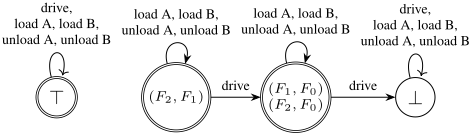
Figure 2 shows the minimized domination LTSs for the fuel factor. The language accepted by starting in a state (si, ti) corresponds to the plans in the domination LTS of that factor. Many cases are fully dominated (e.g. si ⊑LD i ti), and thus are associated with the ⊤ state. The rest are named as the state pairs it is associated with. In the figure, we can see the pattern that was explained before, any state is dominated by a state with less fuel, unless it drives more times than the amount of fuel. For instance, F2 is dominated by F1, unless it does two drive actions. This shows us that the technique discovers the information of the motivating example, as this generalises to more fuel. In particular, the problem might be solvable with one fuel, but the contrastive heuristic will discover that if you have the same state but with one fuel, then the heuristic can be raised to the cost of two drive actions.

5 Qualified Dominance Heuristics

We now consider how to leverage qualified dominance to construct contrastively admissible heuristics. First, we construct a contrastive heuristic based on a node ordering and the perfect heuristic, h∗ . Then, we provide a framework for using any domain-independent heuristic for planning tasks.

5.1 Combining Qualified Dominance Information

Intuitively, we use qualified dominance to exclude plans when estimating the goal-distance of a state. E.g., when computing the heuristic of ns in contrast to nt ∈ N, we want to estimate the goal distance of s excluding the paths in D(s, t).

The first consideration is which nodes from N we can compare to while remaining contrastively admissible. Consider search nodes ns, nt and a path π ∈ D(s, t). We can only disconsider π if we can guarantee that a plan of nt produces a no worse overall plan, i.e. g(ns)+c(π) ≥ g(nt)+h∗ (t). Since c(π) ≥ h∗ (t) this simplifies to g(ns) ≥ g(nt). Taking cost difference into account requires additional analysis. Thus, we use qualified dominance information for a node when considering in contrast to nodes with lower or equal g-value.

We must also avoid circular reasoning. For example, consider search nodes ns and nt with equal g-value, let π ∈ D(s, t) and π′ ∈ D(t, s). Crucially, we cannot disconsider both; it may be that π and π′ are the only optimal plans of s and t, respectively. Therefore, we impose an ordering on the search nodes. Whenever, g(ns) ̸= g(nt) the ordering is easy because the node with larger g-value depends on the one with lower g-value. When g(ns) = g(nt), we assume some arbitrary ordering. In practice, we use the order in which the states are evaluated.

Let ≺ be any strict total order on N satisfying g(n) < g(n′ ) =⇒ n ≺ n′ and n ≺ n′ =⇒ g(n) ≤ g(n′ ), i.e. ≺ respects the g-value ordering and totally orders the nodes. The set of dominated plans for a search node ns in contrast to N given D and ≺ is

where N≺n = { n′ ∈ N | n′ ≺ n } is the lower set of N w.r.t. ≺ and n. The importance of ≺ is that it guarantees that some better plan is always preserved.

Lemma 8. For all π ∈ D≺,D(ns,N), there exists a node nt ∈ N≺ns and a plan π′ ∈ P(t) s.t. π′ ̸∈ D≺,D(nt,N) and c(π′ ) ≤ c(π).

Proof. Let nt be the minimal node in N≺ns w.r.t. ≺ s.t. h∗ (t) ≤ c(π). By Definition 4, such a node exists. Let π′ ∈ P(t) be a plan s.t. c(π′ ) = h∗ (t). Assume that π′ ∈ D≺,D(nt,N). Then there exists nu ∈ N≺nt ⊆ N≺ns s.t. π′ ∈ D(t, u). However, this means that h∗ (u) ≤ c(π′ ) = h∗ (t) and nu ≺ nt, which contradicts the minimality of nt w.r.t. ≺. Thus, π′ ̸∈ D≺,D(nt,N).

We will now define the best possible heuristic for a dominance function and an ordering ≺.

Definition 7. Let D be a qualified dominance function, ns ∈ N and N ⊆ N . The optimal contrastive heuristic w.r.t. D is

Theorem 9. η∗≺,D is contrastively admissible.

Proof. Let nu be a node in N with minimal f ∗ (nu) and among those minimal h∗ (u). Let ns be a node s.t. ns is better than nu (see Def. 2). Since, η∗≺,D takes the minimum over a subset of all plans of s, η∗≺,D (ns,N) ≥ h∗ (s). Assume η∗≺,D (ns,N) > h∗ (s), then there exists a plan π ∈ D≺,D(ns,N) s.t. c(π) = h∗ (s). From Lemma 8, we know that there must then exist a node nt ≺ ns with a plan π′ ̸∈ D≺,D(nt,N) with c(π′ ) ≤ c(π) and thus g(nt) ≤ g(ns) and h∗ (t) ≤ h∗ (s). If f ∗ (ns) < f ∗ (nu) then f ∗ (nt) < f ∗ (nu), which contradicts the minimality of nu. Otherwise, h∗ (s) < h∗ (u) and thus h∗ (t) < h∗ (u), contradicting the minimality of nu. Thus, any node better than nu is admissible, and nu ∈ N is admissible. Thus, η∗≺,D is contrastively admissible.

Importantly, any under-approximation of η∗≺,D is also contrastively admissible. η∗≺,D is also monotonic, however, any under-approximation of η∗≺,D is not necessarily monotonic.

Algorithm 1: Qualified Dominance Heuristic

• 1 Input: A planning task T = (Θ1, . . . ,Θn) and heuristic h 2 Output: A contrastive heuristic function /* Precomputation */ 3 (⊑LD 1 , . . . ,⊑LD n ) ← compute LD simulation on T 4 (Γ1, . . . , Γn) ←compute domination LTSs w.r.t. ⊑LD 5 (Γ1, . . . , Γn) ←determinize, then minimize, and then complement Γ1, . . . , Γn 6 Func Qualified-Dominance-Heuristic(ns,N): 7 ˆ T ← (Θ1, · · · ,Θn) 8 ˆ s ← s 9 forall nt ∈ N≺ns where ∃i ▪ ∀j ̸= i ▪ sj ⊑LD j tj do 10 ˆ T ← ˆ T ◦ Γi 11 ˆ s ← ˆ s ◦ ({(si, ti)}) 12 return h ˆ T (ˆ s)

5.2 Computation in Planning Tasks

We now show how to utilize qualified dominance LTSs to compute heuristics. With a planning task T = (Θ1, . . . , Θn) and a domain-independent admissible heuristic function h, which can be applied to any planning task so that hT (s) is an admissible estimate from s = (s1, . . . , sn) to the goal in ΘT . The idea is that, for each node ns and set of nodes N, we will compute a new planning task ˆ T = (Θ1, . . . ,Θn, . . . ) and state ˆ s = (s1, . . . , sn, . . . ) extending T and s with additional factors that encode information about the qualified dominance of ns compared to N. Then, we can use the contrastive heuristic η≺,Γ,h (ns, N) = h ˆ T (ˆ s).

Algorithm 1 shows the overall process. First, there is a preprocessing phase before the search starts, where we compute a label-dominance simulation, (⊑LD 1 , . . . ,⊑LD n ), and a domination LTS for each factor (Γ1, . . . , Γn), as described in Section 4.2. In each Γ, the plans for the state (si, ti) represent the plans of si which are dominated by plans of ti. When computing a heuristic for ns, we will compare it against states t where sj ⊑ tj for all j ̸= i, i.e., states t that dominate s in all factors except Θi. There, we are interested in extracting information about the plans of si that are not dominated by ti. Therefore, we need the complement of Γi.

Unfortunately, Γi may be non-deterministic. Therefore, we must do a determinization of the transition system first, and then complement the goal states. This is identical to the complementation of a non-deterministic finite automaton, which can be achieved through the power set construction and then swapping goal and non-goal states [Sipser, 2013, p. 55].

The determinization can cause an exponentially larger number of states in the LTS. This can be a bottleneck in some cases, because the heuristic is not computable in polynomial time. A solution is to determinize the LTS by underapproximating it, e.g. by only encoding one response of t. In this paper, we use the full determinization, which is still viable as this is only done once as precomputation. We leave it to future research to study practical methods of approximation.

We have shown how to construct Γi for each factor i. For a node ns, let ni1 t1 . . . nik tk be a sequence of nodes where nij tj ∈ N≺ns and ∀i′ ̸= ij ▪DΓi′ (si′ , ti′ ) = L∗ . We can now take any domain-independent heuristic h that works on factored tasks, and construct the state-contrastive heuristic

where ˆ T = T ◦ (Γi1 , . . . , Γik ) and ˆ s = s ◦ ((s[i1], t1[i1]), . . . , (s[ik], tk[ik])). In other words, we create a copy of Γij for each node nij tj , and we add it as a factor to the planning task. We then evaluate the heuristic for the state where s is concatenated with (s[ij ], tj [ij ]) for each nij tj .

Theorem 10. Let T be a planning task, ≺ a g-value respecting total order of N, and h an admissible heuristic. The heuristic η≺,Γ,h is contrastively admissible.

Proof. FromTheorem5, we know that DΓ(s, t) = PΓ((s, t)) is a qualified dominance function. We prove that η≺,Γ,h is contrastively admissible by showing that η≺,Γ,h (ns,N) ≤ η∗≺,DΓ (ns,N). Let nt ∈ N s.t. all factors other than i are dominated. An admissible heuristic means that hT (s) ≤ min{ c(π) | π ∈ PT (s) }, if s has a plan. For a planning task T and LTS Θ, it holds that PT ◦Θ(s ◦ s′ ) = PT (s) ∩ PΘ(s′ ) for all states s of T and s′ of Θ. Thus, PT ◦Γi (s ◦ (s[i], t[i])) = PT (s) \ D≺,DΓi (s[i], t[i]) and hT ◦Γi (s ◦ (s[i], t[i])) ≤ min { c(π) | π ∈ PT (s) \ D≺,DΓi (s[i], t[i]) } ≤ η∗≺,Γi (s, {t}). This argument can be used inductively for each node in N≺ns .

Theorem11. Let h be a domain-independent heuristic and≺ a g-value respecting total order of N. If hΘ(s) ≤ hΘ◦Θ′ (s ◦ s′ ) for all LTSs Θ,Θ′ and states s, s′ , then η≺,Γ,h is monotonic.

Proof. Recall Def. 3 and the definition of η≺,Γ,h . It follows that if hΘ(s) ≤ hΘ◦Θ′ (s ◦ s′ ), then η≺,Γ,h is also monotonic, because adding more nodes to N causes more LTSs for h.

Clearly, there are practical concerns to consider here as well. Extending the planning task with a number of factors on the order of the nodes expanded so far is too cumbersome in practice. It remains an open research question how to choose the most informative factors to add.

In principle, any domain-independent heuristic can be used with our method. However, heuristics with heavy preprocessing are undesirable, as the planning task changes for each search state. Operator-counting heuristics [Pommerening et al., 2014] are well-suited for this purpose. They model operator usage as a linear program and solve for the minimumcost assignment. Each transition system of the extended task can be encoded as flow constraints and combined with other constraints [Bonet, 2013; Pommerening et al., 2013; Imai and Fukunaga, 2015] to integrate information from new factors with heuristics for the original task.

6 Experiments

We implemented our approach on top of Fast Downward [Helmert, 2006], as a constraint generation method for operator counting heuristics. We complement them with constraints from LM-cut [Helmert and Domshlak, 2009] on the original planning task. Computing the LM-cut constraints for the transformed tasks is not possible in the current implementation, so we use only flow constraints for the new factors. Our technique should be understood as a proof of concept. We do not yet have a practical way to exploit the qualified dominance information. Therefore, we disregard runtime, as that will require further research into practical exploitation methods. Our main objective is to determine whether qualified dominance can produce more useful information to guide search than dominance pruning, which can be understood as a special case of qualified dominance that prunes (assigns a value of infinity) to any state fully dominated in all factors.

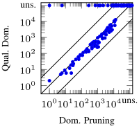
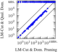
We run experiments with Lab [Seipp et al., 2017] on AMD EPYC 7551 CPUs with memory/time cut-offs of 4 GBs and 30 minutes. We use the Autoscale benchmark set [Torralba et al., 2021], consisting of 42 domains with 30 tasks in each. All tasks are automatically transformed into deterministic FTS tasks [Helmert, 2009; Sievers and Helmert, 2021]. Code and experiment data will be made available upon publication.

The results show that qualified dominance is found on most tasks. The precomputation finishes in 81% of instances, and among those in 93% of cases, we find information over labeldominance simulation (i.e. having more than 3 nodes in the minimal domination LTS). In 79% of the instances where the precomputation finishes, the precomputation time is within a factor of 2 of dominance, and in >99% within a factor of 10. Fig. 3 compares the expansions compared to dominance pruning with the same heuristic. We see a reasonable decrease of expansions in many tasks (e.g., of a factor of 2). Therefore, this can potentially be used for improving heuristic estimates. The combination with LM-cut shows that, even though they are not entirely redundant, the additional constraints are not very complementary to this highly-informed heuristic. This points out the need for further research in how to extract constraints from the additional factors.

7 Conclusion

In this paper, we made two main contributions. First, we introduced contrastive heuristics, which consider the entire search to estimate goal distance from each node, in optimal planning. Second, we presented qualified dominance, a method to identify plans of a state that are dominated by another. We showed how this can be used to enhance heuristics into their contrastive counterpart. While contrastive heuristics based on qualified dominance are not yet practical, this invites further research on extracting heuristic information.

Acknowledgements

This research was partly supported by the Independent Research Fund Denmark through a Sapere Aude: DFF-Starting Grant under reference number 3120-00063B.