
A Novel Local Search Algorithm for the Vertex Bisection Minimization Problem
Proceedings of the Thirty-Fourth International Joint Conference on Artificial Intelligence. Main Track. Pages 8956-8965.
https://doi.org/10.24963/ijcai.2025/996
Keywords
- Search: S: Heuristic search
- Search: S: Local search
Abstract
The vertex bisection minimization problem (VBMP) is a fundamental graph partitioning problem with numerous real-world applications. In this study, we propose a (k, l, S)-cluster guided local search algorithm to address this challenge.
First, we propose a novel (k,l,S)-cluster enumeration procedure, which is based on two key concepts: the (k, l, S)-cluster and the local cluster core. The (k, l, S)-cluster limits both the connectivity and distinct boundaries of a given vertex set, and the local cluster core represents the most cohesive substructure within a (k, l, S)-cluster. Building up on the above (k, l, S)-cluster enumeration procedure, we present a novel (k, l, S)-cluster guided perturbation mechanism designed to escape from local optima.
Next, we propose a two-manner local search procedure that employs two distinct search models to explore the neighboring search space efficiently. Experimental results demonstrate that the proposed algorithm performs best on nearly all instances.
- [Bhatt and Leighton, 1984] Sandeep N Bhatt and Frank Thomson Leighton. A framework for solving vlsi graph layout problems. Journal of Computer and System Sciences, 28(2):300-343, 1984.
- [Brandes and Fleischer, 2009] Ulrik Brandes and Daniel Fleischer. Vertex bisection is hard, too. 2009.
- [Castillo-García and Hernández-Hernández, 2020] Norberto Castillo-García and Paula Hernández-Hernández. Con- structive heuristic for the vertex bisection problem. Journal of applied research and technology, 18(4):187- 196, 2020.
- [Castillo-García and Hernández, 2019] Norberto Castillo- García and Paula Hernández. Two new integer linear programming formulations for the vertex bisection problem. Computational Optimization and Applications, 74(3):895-918, 2019.
- [Chen et al., 2023] Jiejiang Chen, Shaowei Cai, Yiyuan Wang, Wenhao Xu, Jia Ji, and Minghao Yin. Improved local search for the minimum weight dominating set prob- lem in massive graphs by using a deep optimization mech- anism. Artificial Intelligence, 314:103819, 2023.
- [Delling et al., 2011] Daniel Delling, Andrew V Goldberg, Thomas Pajor, and Renato F Werneck. Customizable route planning. In SEA 2011, pages 376-387. Springer, 2011.
- [Fraire et al., 2014] Héctor Fraire, J David Terán-Villanueva, Norberto Castillo García, Juan Javier Gonzalez Barbosa, Eduardo Rodríguez del Angel, and Yazmín Gómez Rojas. Exact methods for the vertex bisection problem. Recent Advances on Hybrid Approaches for Designing Intelligent Systems, pages 567-577, 2014.
- [Herrán et al., 2019] Alberto Herrán, J Manuel Colmenar, and Abraham Duarte. A variable neighborhood search ap- proach for the vertex bisection problem. Information Sci- ences, 476:1-18, 2019.
- [Huacuja and Castillo-García, 2016] Héctor J Fraire Huacuja and Norberto Castillo-García. Optimization of the vertex separation problem with genetic algorithms. In Handbook of Research on Military, Aeronautical, and Maritime Logistics and Operations, pages 13-31. 2016.
- [Jain et al., 2016a] Pallavi Jain, Gur Saran, and Kamal Sri- vastava. Branch and bound algorithm for vertex bisec- tion minimization problem. In ICACCT, pages 17-23. Springer, 2016.
- [Jain et al., 2016b] Pallavi Jain, Gur Saran, and Kamal Sri- vastava. A new integer linear programming and quadrat- ically constrained quadratic programming formulation for vertex bisection minimization problem. Journal of Au- tomation Mobile Robotics and Intelligent Systems, 10, 2016.
- [Jain et al., 2016c] Pallavi Jain, Gur Saran, and Kamal Sri- vastava. On minimizing vertex bisection using a memetic algorithm. Information Sciences, 369:765-787, 2016.
- [Jin et al., 2021] Yan Jin, Bowen Xiong, Kun He, Jin-Kao Hao, Chu-Min Li, and Zhang-Hua Fu. Clustering driven iterated hybrid search for vertex bisection minimiza- tion. IEEE Transactions on Computers, 71(10):2370- 2380, 2021.
- [Kornai and Tuza, 1992] András Kornai and Zsolt Tuza. Narrowness, pathwidth, and their application in natu- ral language processing. Discrete Applied Mathematics, 36(1):87-92, 1992.
- [Luo et al., 2022] Chuan Luo, Wenqian Xing, Shaowei Cai, and Chunming Hu. Nusc: an effective local search algo- rithm for solving the set covering problem. IEEE transac- tions on cybernetics, 54(3):1403-1416, 2022.
- [Malewicz et al., 2010] Grzegorz Malewicz, Matthew H Austern, Aart JC Bik, James C Dehnert, Ilan Horn, Naty Leiser, and Grzegorz Czajkowski. Pregel: a system for large-scale graph processing. In SIGMOD, pages 135- 146, 2010.
- [Newman, 2002] Mark EJ Newman. Assortative mixing in networks. Physical review letters, 89(20):208701, 2002.
- [Shi and Malik, 2000] Jianbo Shi and Jitendra Malik. Nor- malized cuts and image segmentation. IEEE Transactions on pattern analysis and machine intelligence, 22(8):888- 905, 2000.
- [Soto et al., 2022] Carlos Soto, Eduardo Del Ángel- Martínez, Héctor Fraire-Huacuja, Bernabe Dorronsoro, Nelson Rangel, and Laura Cruz-Reyes. Two novel branch and bound algorithms for the vertex bisection problem. Expert Systems with Applications, 190:116169, 2022.
- [Sun et al., 2024] Rui Sun, Yiyuan Wang, HL Shimao Wang, Hui Li, Ximing Li, and Minghao Yin. Nukplex: An effi- cient local search algorithm for maximum k-plex problem. In IJCAI, pages 7029-7037, 2024. IJCAI
- [Terán-Villanueva et al., 2019] J David Terán-Villanueva, Héctor Joaquín Fraire-Huacuja, Salvador Ibarra Martínez, Laura Cruz-Reyes, Jose Antonio Castán Rocha, Clau- dia Gómez Santillán, and Julio Laria Menchaca. Cellu- lar processing algorithm for the vertex bisection problem: Detailed analysis and new component design. Information Sciences, 478:62-82, 2019.
- [Tian et al., 2022] Xinliang Tian, Dantong Ouyang, Rui Sun, Huisi Zhou, and Liming Zhang. Two efficient local search algorithms for the vertex bisection minimization problem. Information Sciences, 609:153-171, 2022.
- [Wang et al., 2020] Yiyuan Wang, Shaowei Cai, Jiejiang Chen, and Minghao Yin. Sccwalk: An efficient lo- cal search algorithm and its improvements for maxi- mum weight clique problem. Artificial Intelligence, 280:103230, 2020.
- [Wu et al., 2015] Qinghua Wu, Yang Wang, and Zhipeng Lü. A tabu search based hybrid evolutionary algorithm for the max-cut problem. Applied Soft Computing, 34:827-837, 2015.
- [Zheng et al., 2025] Jiongzhi Zheng, Kun He, Jianrong Zhou, Yan Jin, Chu-Min Li, and Felip Manyà. Integrating multi-armed bandit with local search for maxsat. Artificial Intelligence, 338:104242, 2025.
References were extracted automatically from the PDF and may contain errors.
Full text extracted automatically from the PDF; figures, tables and equations may differ. The PDF is the version of record.
1 Introduction
The vertex bisection minimization problem (VBMP) is a fundamental graph partitioning problem. It aims to partition the vertex set of a connected graph G into two nearly equal, disjoint subsets, B and B′ , while minimizing the vertex width (VW). The VW is defined as the number of vertices in B that have at least one adjacent vertex in B′ . The VBMP has wide-ranging applications across various fields, including route planning [Delling et al., 2011], very-large-scale integration circuit design [Bhatt and Leighton, 1984], natural language processing [Kornai and Tuza, 1992], image processing [Shi and Malik, 2000], and distributed computing [Malewicz et al., 2010]. Furthermore, the VBMP on general graphs is known to be NP-hard [Brandes and Fleischer, 2009]. Given its theoretical importance and practical applications, the VBMP has attracted significant attention, leading to numerous algorithms to address this problem.
∗Corresponding author
The VBMP algorithms can generally be classified into two main categories: exact algorithms and heuristic algorithms. Exact methods aim to obtain an optimal solution for the VBMP. Fraire et al. [2014] proposed integer linear programming (ILP) models and branch-and-bound algorithms, demonstrating strong performance on small-scale instances. Jain et al. [2016b] later enhanced the efficiency of this work [Fraire et al., 2014] by introducing improved ILP and the models of quadratically constrained quadratic programming. Further work refined branch-and-bound algorithms by incorporating greedy heuristics, significantly reducing execution times, and delivering competitive results in small-scale instances [Jain et al., 2016a]. Furthermore, Castillo-Garc´ıa et al. [2019] developed two new ILP models, expanding both the theoretical framework and the practical efficiency for the VBMP. Soto et al. [2022] proposed two branch-and-bound algorithms for the VBMP. Despite these advancements, the state-of-the-art exact algorithms for the VBMP remain inadequate for solving hard or large-scale instances within a reasonable time frame.
There are several VBMP heuristics and metaheuristics that are commonly used to deliver high-quality solutions with acceptable computational costs. Huacuja et al. [2016] proposed a genetic algorithm to solve the VBMP. Jain et al. [2016c] introduced a memetic algorithm for the VBMP, which integrates four construction heuristics, a specialized crossover operator, and a local improvement operator. Herran et al. [2019] proposed a local search algorithm called BVNS, which outperformed previous methods significantly. The algorithm employs three initialization methods and utilizes two distinct search models, systematically dividing the process into solution construction and improvement phases. Furthermore, cellular processing heuristic methods [Ter´anVillanueva et al., 2019] and greedy randomized adaptive search-based constructive algorithms [Castillo-Garc´ıa and Hern´andez-Hern´andez, 2020] have been proposed to achieve an effective balance between solution quality and computational efficiency. Jin et al. [2021] were the first to introduce learning techniques into heuristic algorithms for the VBMP, proposing a clustering-driven iterated hybrid search algorithmCLUHS. Subsequently, Tian et al. [2022] enhanced the effectiveness of BVNS by incorporating the bucket sorting technique, resulting in two new algorithms including BVNSbucket and BVNSbucket2. Among these heuristic algorithms, CLUHS, BVNSbucket, and BVNSbucket2 achieve the state-of-the-art performance.
In this work, we propose a novel (k, l, S)-cluster guided local search algorithm CELS 1 for the VBMP. It comprises three core components. Experimental results show that the proposed algorithm performs best on almost all instances.
We first introduce two novel concepts: the (k, l, S)-cluster and the local cluster core. Based on these, we propose a new (k, l, S)-cluster enumeration algorithm. The (k, l, S)-cluster integrates two key parameters, k and l, to balance vertex connectivity and boundary distinctiveness within a cluster. Each (k, l, S)-cluster is associated with a local cluster core, which represents the most cohesive substructure within that cluster. By enumerating both the (k, l, S)-clusters and their corresponding local cluster cores, we can identify cohesive substructures in the graph. These substructures then guide subsequent perturbation and local search procedures.
Second, to address the challenge of escaping from local optima, we introduce a novel (k, l, S)-cluster guided perturbation mechanism. This mechanism incorporates the concept of strong correlation relationships between a local cluster core and a (k, l, S)-cluster. Building on this definition and the enumerated (k, l, S)-clusters, the perturbation algorithm groups clusters with similar local structures on the same side (i.e., either B or B′ ). This approach allows the perturbation procedure to guide exploration based on structural patterns, facilitating a more informed and effective search.
Finally, we propose a novel two-manner local search algorithm. The algorithm locks the enumerated local cluster cores to enable deeper exploration within specific search areas. To balance the trade-off between search effectiveness and computational cost, it alternates between coarse-grained and finegrained search modes, depending on the quality of the current solution. By dynamically adjusting its search strategy and thoroughly exploring targeted regions, the algorithm ensures flexibility and adaptability in handling different graph structures.
Section 2 introduces some necessary background knowledge for VBMP. In Section 3, we present the top-level framework of CELS. Section 4 introduces the maximal (k, l, S)- cluster enumeration procedure, followed by the (k, l, S)- cluster-guided perturbation procedure in Section 5. The twomanner local search algorithm is described in Section 6. Experimental results are presented in Section 7, and conclusions are introduced in Section 8.
2 Preliminaries
Given an undirected graph G = (V, E), V = {v1, . . . , vn} is the set of n vertices and E ⊆ V ×V is the set of edges where each edge is represented as a 2-element subset of V . The neighborhood of a vertex v is N(v) = {u ∈ V | (u, v) ∈ E}, and its degree is |N(v)|. We use dmax to denote the maximum degree value of all vertices. The closed neighborhoods of v is defined as N[v] = N(v) ∪ {v}, and N2(v) is the union of the neighborhoods of all vertices in N(v), excluding v, i.e., N2(v) = ⋃u∈N(v) N(u) \ {v}. Given a vertex set S ⊆ V , the induced subgraph G[S] = (VS, ES) is a subgraph of G where VS = S and the edge set ES includes all the edges in E that have both endpoints in S. Given two distinct vertices v1, v2 ∈ V , the similarity between v1 and v2 is defined as the number of vertices in the intersection of their closed neighborhoods, i.e., Simi(v1, v2) = |N[v1] ∩ N[v2]|. Similarly, the difference between v1 and v2 is defined as the number of vertices in the union of their closed neighborhoods that are not included in their intersection, i.e., Diff(v1, v2) = |(N[v1] ∪N[v2]) \ (N[v1] ∩N[v2])|. The variables simi avg and diff avg represent the average similarity and difference values of all distinct vertex pairs in V , respectively.
1 Source code and supplementary materials are available at https://github.com/yiyuanwang1988/CELS.
Given an undirected graph G = (V, E), the VBMP problem focuses on partitioning the vertex set V into two disjoint subsets B and B′ , such that B ∪ B′ = V and B ∩ B′ = ∅. The valid partition D = (B,B′ ) must satisfy the following conditions: if |V | is even, then |B| = |B′ | = |V | 2 ; if |V | is odd, the sizes of B and B′ differ by at most 1, meaning |B| = ⌊ |V | 2 ⌋ and |B′ | = ⌈ |V | 2 ⌉. The objective of the VBMP is to find a valid partition D = (B,B′ ) that minimizes the size of the subset VW(D) ⊆ B, where VW(D) includes all vertices in B that are adjacent to at least one vertex in B′ , i.e., V W(D) = {v ∈ B | ∃u ∈ B′ , (u, v) ∈ E}.
In the local search process, we maintain a valid partition D = (B,B′ ) as the current candidate solution. Local search algorithms for VBMP usually modify the candidate solution D through three basic operators, including Drop, Add, Swap [Herr´an et al., 2019; Tian et al., 2022]. To evaluate the effect of these operations, scoring functions are used to compute the change in the objective value V W(D) resulting from each operator. These operators and their corresponding scoring functions are as follows:
- Drop: The Drop operator moves a vertex v from B to B′ . Formally, the new solution is D1 = (B \ {v},B′ ∪ {v}), and we denote this operation as D1 := drop(v, D).
- Add: The Add operator moves a vertex v from B′ to B. Formally, the resulting solution is D1 = (B ∪ {u},B′ \ {u}), and this operation is represented as D1 := add(u,D).
- Swap: The Swap operator exchanges a vertex v from B with another vertex u from B′ . This results in a new partition D1 = (B \{v}∪{u}, B′ \{u}∪{v}), denoted as D1 := swap(v, u,D).
The scoring functions of the aforementioned operations are used to evaluate the change in the VW value, denoted as ∆drop(D, v), ∆add(D, u), and ∆swap(D, v, u) where v ∈ B and u ∈ B′ , respectively.
3 The Top-Level Framework of the CELS
In this section, we present the top-level framework of CELS in Algorithm 1. The algorithm uses D, Dlb, and Dbest to represent the candidate solution, the local best solution, and the global best solution, respectively. Initially, the algorithm employs the greedy constructive method C1 from BVNS to initialize D and Dbest (Line 1), with further details available
Algorithm 1: CELS
Input: A graph G = (V, E), the cutoff time cutoff
Output: The obtained best solution Dbest
1 D :=Dbest := C1(G);
2 while elapsed time < cutoff do
3
4
5
6
⟨SetS′ , SetS′′ ⟩ := CluEnum(G,D) ;
⟨Dper, Vlock⟩ := CluPer(G, SetS′ , SetS′′ ,D);
⟨D,Dlb⟩ := TwoManner(G,Dper,Dbest, Vlock);
if |VM(Dlb)| < |VM(Dbest)| then Dbest :=Dlb ;
7 return Dbest;
in [Herr´an et al., 2019]. The algorithm then enters a loop that continues until the predefined time limit cutoff is reached (Line 2). In each iteration, the cluster enumeration algorithm is executed to generate the set of (k, l, S)-clusters SetS′ , and the corresponding set of local cluster cores SetS′′ (Line 3), which are presented in Section 4. By using SetS′ and SetS′′ , the algorithm performs the cluster guided perturbation procedure to generate a perturbed solution Dper and obtain the set of locked vertices Vlock (Line 4), which is presented in Section 5. Based on them, the two-manner local search procedure is applied (Line 5), as detailed in Section 6. If the local best solution, Dlb, obtained from the two-manner search is better than the current global best solution, Dbest, it updates Dbest to Dlb (Line 6). Finally, the algorithm returns Dbest (Line 7).
4 The Maximal (k, l, S)-Cluster Enumeration Procedure
Recently, Jin et al. [2021] utilizes an unsupervised machine learning technique based on similarity criteria to divide vertices into clusters and develop a cluster-driven local search algorithm. However, the generated clusters aren't changed throughout the entire local search process. Moreover, the structure of the clusters doesn't account for the differences between vertices or the core structures within clusters. Based on this consideration, we propose the maximal (k, l, S)-cluster enumeration procedure. In this section, we first introduce some key definitions of the (k, l, S)-cluster, and then present the (k, l, S)-cluster generation and enumeration procedures.
4.1 Key Definitions of (k, l, S)-Cluster
Definition 1 ((k, l, S)-Cluster). Given a graph G = (V, E), a vertex set S ⊆ V , and two integer parameters k and l, a (k, l, S)-cluster is defined as a subset S′ ⊆ S such that for every pair of distinct vertices v1, v2 ∈ S′ , Simi(v1, v2) ≥ k and Diff(v1, v2) ≤ l.
Amaximal (k, l, S)-cluster is a subset S′ ⊆ S such that for every pair of distinct vertices v1, v2 ∈ S′ , Simi(v1, v2) ≥ k and Diff(v1, v2) ≤ l, and no vertex can be added to S′ without violating these conditions.
The (k, l, S)-cluster is designed to identify a subset of S that balances overlap and exclusivity within the neighborhoods of the vertices in S. Specifically, the parameter k ensures that pairs of vertices within the cluster share a sufficiently large intersection in their closed neighborhoods, promoting strong local connectivity and cohesion. Meanwhile, the parameter l limits the number of non-shared neighbors, preventing the inclusion of vertices that deviate significantly from the cluster's structure. Together, these conditions enable the (k, l, S)-cluster to maintain both cohesion and clear boundaries.
Given a (k, l, S)-cluster S′ and a vertex vf ∈ V , we utilize simi thre(vf , S′ ) to denote the maximum similarity value between vf and vertices in S′ \ {vf}, i.e., simi thre(vf , S′ ) := maxv′∈S′ \{vf} Simi(vf , v′ ). Besides, we utilize diff thre(vf , S′ ) to denote the minimum difference value between vf and vertices in S′ \ {vf}, i.e., diff thre(vf , S′ ) := minv′∈S′ \{vf} Diff(vf , v′ ). Building on these two definitions, we define two types of local cluster core within a specified local (k, l, S)-cluster.
Definition 2 (Local Similarity Core). Given a graph G = (V,E), a (k, l, S)-cluster S′ and a vertex vf ∈ S′ , a local similarity core of vf is a subset S′′ ⊆ S′ such that vf ∈ S′′ , and for every distinct vertex pair v1, v2 ∈ S′′ , Simi(v1, v2) ≥ simi thre(vf , S′ ).
Definition 3 (Local Difference Core). Given a graph G = (V,E), a (k, l, S)-cluster S′ and a vertex vf ∈ S′ , a local difference core of vf is a subset S′′ ⊆ S′ such that vf ∈ S′′ , and for every distinct vertex pair v1, v2 ∈ S′′ , Diff(v1, v2) ≤ diff thre(vf , S′ ).
Given a (k, l, S)-cluster S′ , the two definitions above impose strong constraints on a specified vertex vf . Specifically, the local similarity core is designed to extract the most cohesive subset containing vf within S′ , focusing on maximizing connectivity. On the other hand, the local difference core identifies the subset of S′ containing vf that minimizes structural divergence, ensuring internal consistency within the cluster.
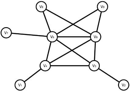
We present an example for the maximal (k, l, S)- cluster and local cluster core in Figure 1. Let S = {v1, v2, v3, v4, v5, v6, v7, v8, v9}. A (2, 4, S)-cluster in Figure 1 is {v3, v4, v5, v6, v8, v9} (denoted as C1), as the similarity between every pair of vertices in this set is at least 2, and the difference between every pair is at most 4. Since no vertices can be added without violating the similarity and difference constraints, C1 is also a maximal (2, 4, S)-cluster. Given C1 and a vertex v6 ∈ C1, the set {v5, v6} is both a local similarity core and a local difference core. This is because {v5, v6} ⊆ C1, Simi(v5, v6) = simi thre(v6,C1), and Diff(v5, v6) = diff thre(v6,C1).
4.2 (k, l, S)-Cluster Generation Algorithm
The (k, l, S)-cluster generation algorithm is detailed in Algorithm 2. To begin with, several necessary variables are introduced: S′ represents the currently generated cluster, and S′′ refers to either the local similarity core or the local difference core of S′ . The input parameters k, l, and S define the constraints for generating the (k, l, S)-cluster S′ , while vf denotes the first vertex to be added to S′ . Additionally, Cand is the set of candidate vertices, where adding any vertex from Cand to S′ ensures that S′ remains a valid (k, l, S)-cluster. The variables simi and diff correspond to the maximum similarity and the minimum difference between vf and Cand, respectively. Lastly, enum pre has two possible values: '1', meaning that the algorithm selects the vertex with the highest Simi value, and '0', indicating a preference for selecting the vertex with the lowest Diff value.
The algorithm begins by initializing various variables or sets as needed (Lines 1-4). It then enters a loop where it iteratively selects a vertex v to add to S′ (Lines 6-13) until Cand becomes empty (Line 5).
If the algorithm enters the similarity phase (i.e., enum pre = 1), for each vertex v ∈ Cand, the algorithm records the lowest similarity value between v and all vertices in S′ . Then, the algorithm selects the vertex v with the highest recorded similarity value (Line 7). If this similarity value between v and all vertices in S′ is not lower than simi, the algorithm adds the selected vertex v to S′′ (Line 8). Otherwise, if enum pre = 0, the algorithm goes into the difference phase. For each vertex v ∈ Cand, the algorithm records the biggest difference value between v and all vertices in S′ again, and selects the vertex v with the smallest recorded difference value (Lines 9-10). If this difference value between v and all vertices in S′ is not greater than diff, v is added to S′′ (Line 11). After each iteration, the algorithm updates both S′ and Cand (Lines 12-13). Finally, when the loop completes, S′ and S′′ are returned (Line 14).
The generation algorithm CluGen is designed to generate a maximal (k, l, S)-cluster S′ . To achieve this, it introduces two vertex selection preferences that result in two types of clusters. The "Similarity" preference focuses on selecting vertices with the highest similarity within S′ , ensuring that the cluster remains tightly connected. In contrast, the "Difference" preference emphasizes selecting vertices with the minimal difference within S′ , which helps to enhance the distinct boundary of the cluster.
4.3 (k, l, S)-Cluster Enumeration Algorithm
Based on the cluster generation algorithm, we develop the (k, l, S)-cluster enumeration algorithm in Algorithm 3.
In this algorithm, SetS′ and SetS′′ are two sets that store the (k, l, S)-clusters and their corresponding local cluster cores generated by the CluGen procedure. Furthermore, we incorporate the concept of assortativity to assist in cluster enumeration. Assortativity measures the tendency of vertices
Algorithm 2: CluGen
Input: Graph G = (V, E), a vertex subset S ⊆ V , a candidate vertex vf ∈ S, enumeration preference enum pre and cluster parameters k and l Output: A maximal (k, l, S)-cluster S′ ⊆ S, a core structure S′′ ⊆ S′ 1 S′ := {vf}, S′′ := ∅; 2 Cand := {v ∈ S | Simi(vf , v) ≥ k, Diff(vf , v) ≤ l}; 3 simi :=maxv′∈Cand Simi(vf , v′ ); 4 diff :=minv′∈Cand Diff(vf , v′ ); 5 while Cand ̸= ∅ do 6 if enum pre = 1 then // Enter into Similarity Phase 7 select a vertex v ∈ Cand with the biggest Simi(v, v′ ) value, breaking ties randomly, where v′ = argminv′∈S′ Simi(v, v′ ); 8 if ∀v′′ ∈ S′ , Simi(v′′ , v) ≥ simi then S′′ := S′′ ∪ {v} ; 9 else // Enter into Difference Phase 10 select a vertex v ∈ Cand with the smallest Diff(v, v′ ) value, breaking ties randomly, where v′ = argmaxv′∈S′ Diff(v, v′ ); 11 if ∀v′′ ∈ S′ , Diff(v′′ , v) ≤ diff then S′′ := S′′ ∪ {v} ; 12 S′ := S′ ∪ {v}; 13 update the Cand accordingly; 14 return ⟨S′ , S′′ ⟩;in a network to connect with others that have similar or dissimilar degrees [Newman, 2002]. A positive assortativity coefficient indicates that high-degree vertices are likely to connect with other high-degree vertices, while a negative coefficient suggests that high-degree vertices tend to connect with low-degree vertices. When the coefficient is 0, the connections are random, with no preference based on degree.
At the beginning, several variables are initialized (Lines 12). Subsequently, the algorithm iteratively calls the CluGen NE times, where NE is a parameter (Lines 3-17). In each iteration, with 50% probability, the algorithm chooses a random vertex vf as the first vertex. Otherwise, the algorithm selects the first vertex vf with the smallest score, further preferring the one with the lowest freq (Lines 4-7). In this context, score(v) is defined as ∆drop(D, v) if v ∈ B, and ∆add(D, v) if v ∈ B′ . Additionally, freq represents the number of times a vertex has been selected as the first vertex during the cluster enumeration process. If the assortativity value of G is not smaller than 0, it indicates that high-degree vertices are likely to connect to other high-degree vertices, and low-degree vertices tend to connect with other low-degree vertices. In such case, high-degree vertices tend to naturally form dense communities. By focusing on similarity, the generated (k, l, S)- cluster takes advantage of this tendency to group highly connected vertices together. Thus, enum pre is set to 1, and the algorithm imposes strong constraints on k and looser constraints on l (Lines 9-11). In detail, k is set to the larger value between simi avg × β and 2, where β is a parameter (Line 10), whereas l is set to maxv∈N2(vf ) Diff(vf , v)-1 (Line 11).
Algorithm 3: CluEnum
Input: Graph G = (V, E), a candidate solution D = (B, B′ ) Output: The cluster collections SetS′ and SetS′′ 1 SetS′ := SetS′′ := ∅; 2 S := V , enum pre := -1; 3 for i = 1 to NE do 4 if with 50% probability then 5 select a random vertex vf ∈ S; 6 else 7 select a vertex vf ∈ S with the smallest score value, further preferring the one with the lowest f req; 8 if Assortativity(G) ≥ 0 then 9 enum pre := 1; 10 k :=max(simi avg ×β, 2); 11 l :=maxv∈N2(vf) Diff(v, vf) -1; 12 else 13 enum pre := 0; 14 k := 1, l := diff avg ×β; 15 ⟨S′ , S′′ ⟩ := CluGen(G, S, vf , enum pre, k, l); 16 S := S \ S′ ; 17 SetS′ := SetS′ ∪ {S′ }, SetS′′ := SetS′′ ∪ {S′′ }; 18 return ⟨SetS′ , SetS′′ ⟩;That is, the algorithm only forbids the vertices in N2(vf ) that has the maximum difference value with vf .
Conversely, if the assortativity value of G is less than 0, it indicates that high-degree vertices tend to connect to lowdegree vertices. In this scenario, the graph does not form well-defined, tightly connected communities. Instead, there are greater structural differences between vertices. In this case, it becomes more meaningful to focus on the differences between the vertices, so the algorithm takes the difference between vertices as the primary consideration factor. Therefore, enum pre is set to 0. The algorithm imposes strong constraints on l and looser constraints on k. In detail, k is set to 1, and l is set to diff avg×β (Line 14).
Subsequently, the algorithm calls the CluGen and then gets the ⟨S′ , S′′ ⟩ (Line 15). Then, S is updated by removing S′ , i.e., S \ S′ (Line 16), ensuring that the vertex cannot exist in different clusters. SetS′ and SetS′′ are updated accordingly (Line 17). Finally, ⟨S′ , S′′ ⟩ is returned (Line 18).
5 The (k, l, S)-Cluster Guided Perturbation Procedure
In this section, we introduce the (k, l, S)-cluster guided perturbation algorithm. First, we introduce the definition of the strong correlation relationship between a local cluster core and another (k, l, S)-cluster as follows:
Definition 4 (Strong Correlation Relationship). Given a graph G = (V, E), two different (k, l, S)-clusters S′ and S′1 such that S′ ∩S′1 = ∅, and a vertex vf ∈ S′ . We consider two situations.
- If Assortativity(G) ≥ 0, we utilize S′′ to denote a local similarity core of vf and S′ . Then, if
- simi thre(vf , S′1 ) ≥ simi thre(vf , S′′ ), then S′′ has a strong correlation relationship with S′1 .
- If Assortativity(G) < 0, we utilize S′′ to denote the local difference core of vf and S′ . Then, if diff thre(vf , S′1 ) ≤ diff thre(vf , S′′ ), then S′′ has a strong correlation relationship with S′1 .
When one of the above conditions is satisfied, the vertex vf and its corresponding local cluster core S′′ show a strong correlation with S′1 , which is denoted as Strong(vf , S′′ , S′1 )=1. If the condition is not met, the correlation is considered absent, and thus Strong(vf , S′′ , S′1 )=0.
If a local cluster core has a strong correlation relationship with another (k, l, S)-cluster, it indicates that they share similar structures. Based on this consideration, we developed the (k, l, S)-cluster guided perturbation algorithm.
Recently, numerous local search algorithms have adopted the lock-unlock mechanism to explore specific search areas more deeply [Jin et al., 2021; Chen et al., 2023], and employed perturbation strategies to escape from local optima [Wang et al., 2020; Sun et al., 2024]. This study also integrates these strategies to strengthen the search process through deep exploration of the search space and robust mechanisms for escaping local optima. Specifically, in the perturbation and local search procedures, vertices can be in one of two states: locked or unlocked, with only unlocked vertices being movable. During the local search process, when the algorithm becomes trapped in local optima, it uses heuristic methods to move the vertices.
The locked vertices are those within the enumerated local cluster cores, each of which is locked in either B or B′ . The vertices moved during the perturbation procedure are those located within the enumerated (k, l, S)-clusters. This is because the local cluster cores represent the most cohesive components within the given (k, l, S)-cluster, so we lock them in the entire local search procedure. As for the perturbation, it aims to explore the search space more broadly and escape local optima. To achieve this, the algorithmmodifies the current solution by moving the entire (k, l, S)-cluster.
During the perturbation procedure, we use Vlock to denote the set of locked vertices. The local cluster cores locked in B and B′ are represented by CoreB and CoreB′ , respectively. We use the flag variable to determine whether a local cluster core is locked in B or B′ . Specifically, flag = 0 means that the core is locked in B, while flag = 1 indicates it is locked in B′ .
The algorithm is outlined in Algorithm 4. Initially, Vlock, CoreB and CoreB′ are set to ∅ (Line 1). Then, the algorithm iteratively transverse the enumerated (k, l, S)-clusters and their corresponding local cluster cores NE times (Lines 2-28). In the i-th iteration, the i-th enumerated cluster and local cluster core are extracted as S′ i and S′′ i , respectively (Lines 3-4). If the |S′′ i | is not larger than 1, the algorithm skips the current iteration (Line 5). The vertex vf , which was first added to S′′ i , is then extracted (Line 6). Next, the algorithm determines whether S′′ i is locked in B or B′ . Specifically, if there exists a local cluster core S′′ core in B that has a strong relationship with S′′ i , but no local cluster core in B′ exhibits a strong relationship with S′′ i , we set flag to 0. Con-
Algorithm 4: CluPert
Input: Graph G = (V, E), the set of (k, l, S)-clusters SetS′ , the set of local cluster cores SetS′′ , candidate solution D Output: The perturbed solution D 1 Vlock := CoreB := CoreB′ = ∅; 2 for i = 1 to NE do 3 S′ i :=select the ith element in SetS′ ; 4 S′′ i :=select the ith element in SetS′′ ; 5 if |S′′ i | ≤ 1 then continue; 6 extract the vertex vf that was first added to S′′ i ; 7 CanB := {S′′ c ∈ CoreB | Strong(vf , S′′ i , S′′ c ) = 1}; 8 CanB′ :={S′′ c ∈ CoreB′ | Strong(vf , S′′ i , S′′ c ) = 1}; 9 if CanB ̸= ∅ and CanB′ = ∅ then 10 flag := 0; 11 else if CanB = ∅ and CanB′ ̸= ∅ then 12 flag := 1; 13 else 14 flag := select a random value from {0, 1}; 15 if flag = 0 then 16 move count := |S′ i \ B|; 17 B := B ∪ S′ i; 18 for i = 1 to move count do 19 v∗ := argminv∈B\Vlock ∆drop (D, v); 20 D := drop(v∗ ,D) ; 21 Vlock := Vlock ∪S′′ i , CoreB := CoreB ∪ {S′′ i }; 22 else 23 move count := |S′ i \ B′ |; 24 B′ := B′ ∪S′ i; 25 for i = 1 to move count do 26 v∗ := argminv∈B′\Vlock ∆add (D, v); 27 D := add(v∗ ,D) ; 28 Vlock := Vlock ∪S′′ i , CoreB′ := CoreB′ ∪ {S′′ i }; 29 return ⟨D, Vlock⟩;versely, if there exists a local cluster core S′′ core in B′ with a strong relationship to S′′ i , but no such local cluster core exits in B, we set flag to 1. Otherwise, flag is set to a random value from 0 and 1. Note that each local cluster core stored in CoreB or CoreB′ is also considered as a (k, l, S)-cluster. In this mechanism, if a local cluster core exhibits a strong correlation with another local cluster core, they are considered to have similar substructures and are more likely to be positioned on the same side (i.e., B or B′ ).
Subsequently, if flag equals 0, all vertices in S′ i \ B are moved to B (Line 17). Then, an equal number of vertices are removed from B \ Vlock to B′ , specifically by removing the vertex v with the highest ∆drop(D, v) from the unlocked vertices (Lines 18-20). After this, Vlock and CoreB are updated accordingly (Line 21). If flag is 1, all vertices in S′ i \ B′ are moved to B′ (Line 24). Then, an equal number of vertices are removed from B′ \Vlock to B, again by removing the vertex v with the highest ∆add(D, v) from the unlocked vertices (Lines 25-27). Vlock and CoreB′ are updated accordingly (Line 28). Finally, the perturbed solution D and the locked set Vlock are returned (Line 29).
6 Two-Manner Local Search Algorithm
In this section, we present the two-manner local search algorithm, including coarse-grained search and fine-grained search manners. First, we review previous search manners for the VBMP and analyze their time complexity. Then, we introduce the swap vertices selection rule utilized in the algorithm. Finally, we present the two-manner local search algorithm.
6.1 Previous SearchManners for the VBMP
Previous local search algorithms typically employ two types of local search manners: the drop&add operations [Herr´an et al., 2019; Tian et al., 2022; Jin et al., 2021] and the swap operation [Herr´an et al., 2019; Tian et al., 2022]. These manners differ in how to select vertices. In the drop&add operation, a vertex v ∈ B with the lowest ∆drop(D, v) is first dropped to B′ , and then a vertex u ∈ B′ with the lowest ∆add(D, u) is selected to be added to B. The swap operation simultaneously selects a vertex v ∈ B and a vertex u ∈ B′ with the lowest ∆swap(D, v, u), and then swaps them. Although the swap operation consistently yields equal or better solution quality compared to the drop&add method [Jin et al., 2021], it has significantly higher time complexity. We analysis their time complexity as follows:
In the local search procedure, ∆swap of each vertex pair can not be maintained in the local search because it requires significant time complexity. But the two local search manners both maintain the ∆drop values of vertices in B and the ∆add values of vertices in B′ in the whole local search procedure. When a vertex v ∈ B and a vertex u ∈ B′ are swapped, both of the two local search manners need to have a complexity of d2max to update ∆drop and ∆add.
The time complexity of their vertex selection procedures differs. Note that the ∆drop values of vertices in B and ∆add values of vertices in B′ are maintained during the local search. By utilizing bucket sorting technique [Tian et al., 2022; Jin et al., 2021], the vertex selection of the drop&add method has a time complexity of O(1). As for the swap operation, the swapped vertex pair are selected by calculating the ∆swap(D, v, u) of each distinct vertex pair v ∈ B and u ∈ B′ , and choosing the best pair among them. According to the study [Tian et al., 2022], for v ∈ B and u ∈ B′ , calculating the ∆swap(D, v, u) has a time complexity of O(dmax). As a result, the vertex selection for the swap operation has a time complexity of O(|B| × |B′ | × |dmax|) = O(|V |2 × |dmax|). This introduces a trade-off between search effect and time consumption. However, previous studies typically execute the swap operation periodically, without exploring a more heuristic approach to deal with the trade-off.
6.2 Swap Vertices Selection Rule
Due to the significant time consumption of the swap operation, we only conduct swap operation for high-quality vertex pairs and select the best pair among them. We then propose the swap vertex selection rule as follows.
Swap Rule. We store the vertices with the highest ∆drop(D, v) fromB\Vlock in SB, and those with the highest ∆add(D, v) fromB′ \Vlock in SB′ . If either set contains more than K vertices, we randomly reserve K vertices in the corresponding set, where K is a parameter. Then, we choose a pair
Algorithm 5: TwoManner
Input: Graph G = (V, E), candidate solution D, the global best solution Dbest, the set of locked vertices Vlock. Output: Local best solution Dlb 1 unimprove := 0, Dlb :=D, step := 0; 2 fb[vi] := 0, for each vertex vi ∈ V ; 3 len :=min(|B \ Vlock|, |B′ \ Vlock|); 4 while unimprove ≤ |V | - |Vlock| do 5 if |VM(D)| ≤ VM(Dbest) then 6 select two vertex v, u according to Swap Rule; 7 D := swap(v, u, D); 8 obtain a random integer inter from ( len 2 , len); 9 fb[v] := step + inter; 10 else 11 select a vertex v ∈ B \ Vlock with the smallest ∆drop(D, v) and fb[v] < step, breaking ties randomly; 12 D := drop(v, D); 13 obtain a random integer inter from (1, len); 14 fb[v] := step + inter; 15 select a vertex u ∈ B′ \ Vlock with the smallest ∆add(D, u) and fb[u] < step, breaking ties randomly; 16 D := add(u, D); 17 unimprove := unimprove + 1, step := step + 1 ; 18 if |VW(D)| < |VW(Dlb)| then 19 Dlb :=D, unimprove := 0; 20 return ⟨D,Dlb⟩;of vertices (v, u) := argminv∈SB,u∈SB′ ∆swap(D, v, u), breaking ties randomly.
In this vertices selection rule, we regard vertices in SB and SB′ as high-quality vertices, and only calculate the score for combinations of these vertices. The time complexity of this vertex selection rule is O(|dmax|). In our algorithm, we set the K as 4, which indicates its time complexity is significancy smaller than previous vertices swap vertices selection rule in most cases. According to our experiments, the in 91.2% cases, the proposed swap rule can swap a better vertex pair than the drop&add operation.
6.3 Details of Two-Manner Local Search
We present the two-manner local search in Algorithm 5, where in each iteration, the algorithm performs either a coarse-grained search (using the drop&add operation) or a fine-grained search (using the swap operation), depending on the quality of the current solution.
The variables step and unimprove track the number of steps taken in the current search and the number of steps in which Dlb has not been improved, respectively. Additionally, len denotes the minimum value between |B \ Vlock| and |B′ \ Vlock|, which incorporates a tabu mechanism [Luo et al., 2022] to prevent cycling issues. Specifically, each vertex is assigned a forbidden variable fb, which increases within a specific range based on the current step after a drop operation. A candidate vertex can only be added back once its forbidden value exceeds the current step.
Initially, the variables unimprove, Dlb, step, and fb are initialized (Lines 1-2). The variable len is set to min(|B \ Vlock|, |B′ \ Vlock|), which is tied to the forbidden status of vertices (Line 3). Then, the algorithm uses either the drop&add or swap operation to explore the neighboring search space of D. If |VM(D)| ≤ VM(Dbest), the finegrained search is conducted by selecting a pair of vertices based on the swap rule and performing the swap operation (Lines 5-7). The algorithm then forbids the dropped vertex v more strongly (Lines 8-9) to account for its greedy selection.
Otherwise, the coarse-grained search is employed to explore the neighboring search space efficiently. An unlocked and unforbidden vertex v is selected greedily from B and moved to B′ (Lines 11-12), after which v is forbidden with a weaker strength (Lines 13-14). Then, an unlocked and unforbidden vertex u is selected from B′ and moved to B (Lines 15-16). The values of unimprove and step are updated accordingly (Line 17). At the end of each loop, if D is better than Dlb, Dlb is updated to D, and unimprove is reset to 0 (Lines 18-19). Finally, if unimprove reaches |V | - |Vlock|, D and Dlb are returned (Line 20).
7 Experiments
In this section, we conduct experiments to evaluate the effectiveness of the proposed algorithm and its key components.
Based on the literature, we compare all the state-of-theart algorithms for the VBMP, including BVNS [Herr´an et al., 2019], BVNSbucket [Tian et al., 2022], BVNSbucket2 [Tian et al., 2022], and CLUHS [Jin et al., 2021]. Among these, CLUHS is the best-performing heuristic algorithm for the VBMP. We compare CELS with these four heuristic algorithms, as well as with the best results reported in previous studies. The source codes for all algorithms are provided by the respective authors.
Following the experiment settings of the previous work [Jin et al., 2021], the time limit is set to 100 seconds. The random seeds are set from 1 to 10. All the algorithms are implemented in C++ and compiled by g++ with '-O3' option. For all competitors, we use the parameters specified in the corresponding literature, while also optimizing these parameters for newly introduced instances. All experiments are conducted on Intel(R) Xeon(R) Platinum 6238 CPU @2.10GHz with 256GB RAM under Ubuntu 22.04.4 LTS.
We select all instances previously adopted by the state-ofthe-art heuristic algorithms. Specifically, [Jin et al., 2021] uses 137 instances, while [Tian et al., 2022] uses 142 instances, many of which overlap with the 137 instances used by CLUHS. After removing the duplicate instances, we collect a total of 243 unique instances. Additionally, 71 large instances are selected from the datasets for the max-cut problem, which is another fundamental graph partitioning problem. We divide the 314 instances into three benchmarks. First, the 71 large graphs are designated as the max-cut-large benchmark [Wu et al., 2015]. Among the remaining 243 instances, 178 with fewer than 500 vertices are classified as the classic medium benchmark, while the remaining 65 instances with more than 500 vertices are categorized as classic large benchmark. According to our preliminary experiments, we set the parameters as NE = 3, β = 0.4, K = 4.
| Benchmark | #ins | CELS #min(#avg) | BVNSBucket #min(#avg) | BVNSBucket2 #min(#avg) | CLHUS #min(#avg) | BVNS #min(#avg) |
|---|---|---|---|---|---|---|
| max-cut-large | 71 | 62(61) | 18(12) | 19(16) | 25(23) | 10(8) |
| classic medium | 178 | 177(169) | 170(163) | 170(166) | 161(148) | 169(157) |
| classic large | 65 | 64(51) | 50(34) | 53(36) | 47(32) | 48(26) |
| #total | 314 | 303(281) | 238(209) | 242(218) | 233(203) | 227(191) |
| Benchmark | #inst. | vs. CELS1 #bet(#wor) | vs. CELS2 #bet(#wor) | vs. CELS3 #bet(#wor) | vs. CELS4 #bet(#wor) | vs. CELS5 #bet(#wor) | vs. CELS6 #bet(#wor) | vs. CELS7 #bet(#wor) |
|---|---|---|---|---|---|---|---|---|
| classic medium | 178 | 2(0) | 1(0) | 7(3) | 0(0) | 2(1) | 15(0) | 3(0) |
| classic large | 65 | 12(0) | 13(0) | 4(1) | 6(3) | 7(2) | 19(0) | 14(1) |
| max-cut-large | 71 | 7(1) | 19(0) | 6(0) | 31(5) | 21(3) | 42(2) | 44(0) |
7.1 Experimental Results on All Benchmarks
The summarized results are presented in Table 1. Detailed results are provided in the supplementary material. In detail, CELS outperforms CLUHS, BVNSbucket, BVNSbucket2, and BVNS in terms of the best solution for 76, 76, 72, and 87 instances, respectively. It is surpassed by CLUHS, BVNSbucket, BVNSbucket2, and BVNS in only 3, 6, 7, and 2 instances, respectively. Moreover, we regard the best results from the results of comparative algorithms and previous results as the best-recorded results. When comparing with the best-recorded results, CELS achieves 50 record-breaking solutions, while it is defeated by those the best-recorded for 11 instances. Regarding average solutions, CELS achieves the best average in 281 out of 314 instances, while BVNS, BVNSbucket, BVNSbucket2, and CLUHS achieve 203, 209, 218, and 191 best average solutions out of 314 instances, respectively. These results clearly highlight the state-of-the-art performance of CELS.
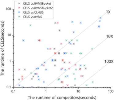
Moreover, we evaluate the runtime performance of the CELS algorithm against three competing methods, focusing on instances where all algorithms achieve identical best and average solution values. To ensure meaningful comparisons, instances with runtimes under 0.1 seconds for both CELS and its competitors are excluded. As illustrated in Figure 2, CELS consistently outperforms its rivals in terms of runtime across the majority of instances.
7.2 Further Results with Exact Algorithms
According to the literature [Castillo-Garc´ıa and Hern´andez, 2019; Soto et al., 2022], the state-of-the-art exact algorithms for the VBMP include ILPVBP and MILP [Castillo-Garc´ıa and Hern´andez, 2019], as well as BBVBP-IVM and BBVBPS [Soto et al., 2022].
First, we compare CELS with ILPVBP and MILP [Castillo-Garc´ıa and Hern´andez, 2019] on all the instances tested in this study, using CPLEX 22.10 as the ILP solver. CELS is tested under a 100s limit and seed 1, while the ILP algorithms are tested under a 1000s limit. Results show CELS outperforms ILPVBP on 74 instances and MILP on 80 instances, while being surpassed by them on only 6 and 5 instances, respectively. The results show that CELS clearly outperforms the two algorithms.
As for the comparison with BBVBP-IVM and BBVBP-S, their source code is not publicly available. Therefore, we compare the results obtained by CELS under a 100-second time limit and seed 1 with the results reported in the literature, where both BBVBP-IVM and BBVBP-S were run for 96 hours. Among the 27 instances used in [Soto et al., 2022], CELS outperforms both BBVBP-IVM and BBVBP-S on 23 instances and is not outperformed on any instance. This comparison further highlights the superior performance of CELS.
7.3 Strategies Analysis of CELS
We generate the following alternative versions of CELS to validate its key ideas: CELS1 and CELS2 discard the assortativity of the graph, with eunm pre consistently set to 0 and 1, respectively. CELS3 does not account for the strong correlation between local cluster cores and randomly displays the (k, l, S)-cluster in B or B′ . CELS4 does not lock the vertices in the local cluster cores. CELS5 only moves the local core clusters without altering the entire (k, l, S)-cluster during the perturbation process. CELS6 and CELS7 only utilize the coarse-grained search or the fine-grained search in the two-manner based local search, respectively. The results in Table 2 show that all the proposed strategies play an important rule in CELS. Moreover, we conduct a more deeply strategy analysis of the two-manner local search. We present this part in the supplementary material.
8 Conclusion
In this paper, we propose a novel local search algorithm named CELS to deal with the VBMP. We propose the definition of the (k, l, S)-cluster and develop the (k, l, S)-cluster enumeration procedure. Based on this procedure, we propose a (k, l, S)-cluster guided perturbation mechanism and the two-manner local search procedure. Experimental results clearly demonstrate that the proposed CELS algorithm achieves the best performance on almost all instances.
In further work, we believe that CELS can be enhanced by optimizing the transition condition between fine-grained and coarse-grained searches. To achieve this, we plan to introduce additional shift conditions and apply a multi-armed bandit [Zheng et al., 2025] approach to dynamically select the most suitable condition for each specific graph.
Acknowledgments
This work is supported by National Cryptologic Science Fund of China 2025NCSF02046, NSFC under Grant No. 61806050 and 62372093, the Fundamental Research Funds for the Central Universities 2412023YQ003, Jilin Science and Technology Department 20240602005RC.
@inproceedings{ijcai2025p996,
  title     = {A Novel Local Search Algorithm for the Vertex Bisection Minimization Problem},
  author    = {Sun, Rui and Wang, Xinyu and Wang, Yiyuan and Li, Jiangnan and Zhou, Yi},
  booktitle = {Proceedings of the Thirty-Fourth International Joint Conference on
               Artificial Intelligence, {IJCAI-25}},
  publisher = {International Joint Conferences on Artificial Intelligence Organization},
  editor    = {James Kwok},
  pages     = {8956--8965},
  year      = {2025},
  month     = {8},
  note      = {Main Track},
  doi       = {10.24963/ijcai.2025/996},
  url       = {https://doi.org/10.24963/ijcai.2025/996},
}
TY - CPAPER TI - A Novel Local Search Algorithm for the Vertex Bisection Minimization Problem AU - Sun, Rui AU - Wang, Xinyu AU - Wang, Yiyuan AU - Li, Jiangnan AU - Zhou, Yi T2 - Proceedings of the Thirty-Fourth International Joint Conference on Artificial Intelligence, IJCAI-25 PB - International Joint Conferences on Artificial Intelligence Organization PY - 2025 SP - 8956 EP - 8965 DO - 10.24963/ijcai.2025/996 UR - https://doi.org/10.24963/ijcai.2025/996 ER -Copied
Machine-readable versions of this paper, for tools and AI agents:





