
NuMDS: An Efficient Local Search Algorithm for Minimum Dominating Set Problem
Proceedings of the Thirty-Fourth International Joint Conference on Artificial Intelligence. Main Track. Pages 8966-8976.
https://doi.org/10.24963/ijcai.2025/997
Keywords
- Search: S: Combinatorial search and optimisation
Abstract
The minimum dominating set (MDS) problem is a crucial NP-hard combinatorial optimization problem with wide applications in real-world scenarios. In this paper, we propose an efficient local search algorithm namely NuMDS to solve the MDS, which comprises three key ideas. First, we introduce a dominate propagation-based reduction method that fixes a portion of vertices in a given graph. Second, we develop a novel two-phase initialization method based on the decomposition method. Third, we propose a multi-stage local search procedure, which adopts three different search manners according to the current stage of the search. We conduct extensive experiments to demonstrate the outstanding effectiveness of NuMDS, and the results clearly indicate that NuMDS outperforms previous state-of-the-art algorithms on almost all instances.
- [Alber et al., 2004] Jochen Alber, Michael R Fellows, and Rolf Niedermeier. Polynomial-time data reduction for dominating set. Journal of the ACM (JACM), 51(3):363- 384, 2004.
- [Alber et al., 2005] Jochen Alber, Hongbing Fan, Michael R. Fellows, Henning Fernau, Rolf Niedermeier, Fran Rosa- mond, and Ulrike Stege. A refined search tree technique for dominating set on planar graphs. Journal of Computer and System Sciences, 2005.
- [Alber et al., 2006] Jochen Alber, Nadja Betzler, and Rolf Niedermeier. Experiments on data reduction for optimal domination in networks. Annals of Operations Research, 146(1):105-117, 2006.
- [Bouamama and Blum, 2015] Salim Bouamama and Chris- tian Blum. A randomized population-based iterated greedy algorithm for the minimum weight dominating set prob- lem. In ICICS, pages 7-12. IEEE, 2015.
- [Cai et al., 2020] Shaowei Cai, Wenying Hou, Yiyuan Wang, Chuan Luo, and Qingwei Lin. Two-goal local search and inference rules for minimum dominating set. In IJCAI, pages 1467-1473, 2020. IJCAI
- [Cai, 2015] Shaowei Cai. Balance between complexity and quality: Local search for minimum vertex cover in massive graphs. In Qiang Yang and Michael J. Wooldridge, editors, IJCAI, pages 747-753, 2015. IJCAI
- [Campan et al., 2015] Alina Campan, Traian Marius Truta, and Matthew Beckerich. Fast dominating set algorithms for social networks. In MAICS, pages 55-62, 2015.
- [Chalupa, 2017] David Chalupa. An order-based algorithm for minimum dominating set with application in graph mining. Information Sciences, 426:101-116, 2017.
- [Chalupa, 2018] David Chalupa. An order-based algorithm for minimum dominating set with application in graph mining. Information Sciences, 426:101-116, 2018.
- [Chaurasia and Singh, 2015] Sachchida Nand Chaurasia and Alok Singh. A hybrid evolutionary algorithm with guided mutation for minimum weight dominating set. Applied In- telligence, 43(3):512-529, 2015.
- [Chen et al., 2007] Jianer Chen, Henning Fernau, Iyad A Kanj, and Ge Xia. Parametric duality and kernelization: Lower bounds and upper bounds on kernel size. SIAM Journal on Computing, 37(4):1077-1106, 2007.
- [Chen et al., 2023] Jiejiang Chen, Shaowei Cai, Yiyuan Wang, Wenhao Xu, Jia Ji, and Minghao Yin. Improved local search for the minimum weight dominating set prob- lem in massive graphs by using a deep optimization mech- anism. Artificial Intelligence, 314:103819, 2023.
- [Dinur and Steurer, 2014] Irit Dinur and David Steurer. An- alytical approach to parallel repetition. In STOC, pages 624-633, 2014.
- [Downey and Fellows, 1995] Rod G Downey and Michael R Fellows. Fixed-parameter tractability and completeness i: Basic results. SIAM Journal on computing, 24(4):873- 921, 1995.
- [Drange et al., 2014] Pål Grønås Drange, Markus S Dregi, Fedor V Fomin, Stephan Kreutzer, Daniel Lokshtanov, Marcin Pilipczuk, Michał Pilipczuk, Felix Reidl, Saket Saurabh, Fernando Sánchez Villaamil, et al. Kernelization and sparseness: the case of dominating set. arXiv preprint arXiv:1411.4575, 2014.
- [Eubank et al., 2004] Stephen Eubank, VS Anil Kumar, Madhav V Marathe, Aravind Srinivasan, and Nan Wang. Structural and algorithmic aspects of massive social net- works. In ACM-SIAM, pages 718-727, 2004.
- [Fan et al., 2019] Yi Fan, Yongxuan Lai, Chengqian Li, Nan Li, Zongjie Ma, Jun Zhou, Longin Jan Latecki, and Kaile Su. Efficient local search for minimum dominating sets in large graphs. In DASFAA, pages 211-228. Springer, 2019.
- [Friedman, 1937] Milton Friedman. The use of ranks to avoid the assumption of normality implicit in the analysis of variance. Journal of the American Statistical Associa- tion, 32(200):675-701, 1937.
- [Garcıa and Herrera, 2008] Salvador Garcıa and Francisco Herrera. An extension on "statistical comparisons of clas- sifiers over multiple data sets" for all pairwise compar- isons. Journal of Machine Learning Research, 9:2677- 2694, 2008.
- [Giap and Ha, 2014] Cu Nguyen Giap and Dinh Thi Ha. Par- allel genetic algorithm for minimum dominating set prob- lem. In ICAC, 2014.
- [Grandoni, 2004] Fabrizio Grandoni. Exact Algorithms for Hard Graph Problems. PhD thesis, Università di Roma 'Tor Vergata', Roma, Italy, 2004.
- [Grandoni, 2006] Fabrizio Grandoni. A note on the com- plexity of minimum dominating set. Journal of Discrete Algorithms, 4(2):209-214, 2006.
- [Guo and Niedermeier, 2007] Jiong Guo and Rolf Nieder- meier. Linear problem kernels for np-hard problems on planar graphs. In ICALP, pages 375-386. Springer, 2007.
- [Gurobi Optimization, 2021] LLC Gurobi Optimization. Gurobi optimizer reference manual. 2021.
- [Hedar and Ismail, 2010a] Abdel-Rahman Hedar and Rashad Ismail. Hybrid genetic algorithm for minimum dominating set problem. In ICCSA, pages 457-467.
- [Hedar and Ismail, 2010b] Abdel-Rahman Hedar and Rashad Ismail. Hybrid genetic algorithm for minimum dominating set problem. In ICCSA, pages 457-467.
- [Hedar and Ismail, 2012] Abdel-Rahman Hedar and Rashad Ismail. Simulated annealing with stochastic local search for minimum dominating set problem. International Jour- nal of Machine Learning and Cybernetics, 3(2):97-109, 2012.
- [Ho et al., 2006] Chin Kuan Ho, Yashwant Prasad Singh, and Hong Tat Ewe. An enhanced ant colony optimization metaheuristic for the minimum dominating set problem. Applied Artificial Intelligence, 20(10):881-903, 2006.
- [Jiang and Zheng, 2023] Hua Jiang and Zhifei Zheng. An exact algorithm for the minimum dominating set problem. In IJCAI, pages 5604-5612, 2023. IJCAI
- [Jovanovic et al., 2010] Raka Jovanovic, Milan Tuba, and Dana Simian. Ant colony optimization applied to mini- mum weight dominating set problem. In ICCAS, 2010.
- [Kitsak et al., 2010] Maksim Kitsak, Lazaros K Gallos, Shlomo Havlin, Fredrik Liljeros, Lev Muchnik, H Eu- gene Stanley, and Hernán A Makse. Identification of in- fluential spreaders in complex networks. Nature physics, 6(11):888-893, 2010.
- [Liu et al., 2011] Yang-Yu Liu, Jean-Jacques Slotine, and Albert-László Barabási. Controllability of complex net- works. nature, 473(7346):167, 2011.
- [López-Ibáñez et al., 2016] Manuel López-Ibáñez, Jérémie Dubois-Lacoste, Leslie Pérez Cáceres, Mauro Birattari, and Thomas Stützle. The irace package: Iterated racing for automatic algorithm configuration. Operations Research Perspectives, 3:43-58, 2016.
- [Okumus ¸and Karcı, 2024] Fatih Okumus ¸and S ¸eyda Karcı. Mdsa: A dynamic and greedy approach to solve the minimum dominating set problem. Applied Sciences, 14(20):9251, 2024.
- [Potluri and Bhagvati, 2012] Anupama Potluri and Chakravarthy Bhagvati. Novel Morphological Algo- rithms for Dominating Sets on Graphs with Applications to Image Analysis. 2012.
- [Potluri and Singh, 2011] Anupama Potluri and Alok Singh. Two hybrid meta-heuristic approaches for minimum dom- inating set problem. In SEMCCO, pages 97-104. Springer, 2011.
- [Potluri and Singh, 2013] Anupama Potluri and Alok Singh. Hybrid metaheuristic algorithms for minimum weight dominating set. Applied Soft Computing Journal, 13(1):76-88, 2013.
- [Raz and Safra, 1997] Ran Raz and Shmuel Safra. A sub- constant error-probability low-degree test, and a sub- constant error-probability pcp characterization of np. In UIST, 1997.
- [Reixach and Blum, 2024] Jaume Reixach and Christian Blum. Extending cmsa with reinforcement learning: Ap- plication to minimum dominating set. In MIC, pages 354- 359. Springer, 2024. [Romania, 2010] Qatar Serbia Romania. Ant colony opti- mization applied to minimum weight dominating set prob- lem. In WSEAS, pages 29-31, 2010.
- [Rossi and Ahmed, 2015] Ryan Rossi and Nesreen Ahmed. The network data repository with interactive graph analyt- ics and visualization. In AAAI, volume 29, 2015.
- [Sanchis, 2002] Laura A Sanchis. Experimental analysis of heuristic algorithms for the dominating set problem. Algo- rithmica, 33:3-18, 2002.
- [Shen and Li, 2010] Chao Shen and Tao Li. Multi-document summarization via the minimum dominating set. In COL- ING, pages 984-992. Coling, 2010.
- [Stefan, 2014] Wuchty Stefan. Controllability in protein interaction networks. Proc Natl Acad Sci U S A, 111(19):7156-7160, 2014.
- [Stojmenovic et al., 2002] Ivan Stojmenovic, Mahtab Sed- digh, and Jovisa Zunic. Dominating sets and neighbor elimination-based broadcasting algorithms in wireless net- works. IEEE Transactions on parallel and distributed sys- tems, 13(1):14-25, 2002.
- [Takaguchi et al., 2014] Taro Takaguchi, Takehisa Hasegawa, and Yuichi Yoshida. Suppressing epidemics on networks by exploiting observer nodes. Physical Review E, 90(1):012807, 2014.
- [Van Rooij and Bodlaender, 2011] Johan MM Van Rooij and Hans L Bodlaender. Exact algorithms for dominating set. Discrete Applied Mathematics, 159(17):2147-2164, 2011.
- [Wang et al., 2017] Yiyuan Wang, Shaowei Cai, and Ming- hao Yin. Local search for minimum weight dominating set with two-level configuration checking and frequency based scoring function. Journal of Artificial Intelligence Research, 58:267-295, 2017.
- [Wang et al., 2018] Yiyuan Wang, Shaowei Cai, Jiejiang Chen, and Minghao Yin. A fast local search algorithm for minimum weight dominating set problem on massive graphs. In IJCAI, pages 1514-1522, 2018. IJCAI
- [Wang et al., 2020] Yiyuan Wang, Shaowei Cai, Jiejiang Chen, and Minghao Yin. Sccwalk: An efficient lo- cal search algorithm and its improvements for maxi- mum weight clique problem. Artificial Intelligence, 280:103230, 2020.
- [Wu, 2002] Jie Wu. Extended dominating-set-based rout- ing in ad hoc wireless networks with unidirectional links. IEEE Transactions on Parallel and Distributed Systems, 13(9):866-881, 2002.
- [Xiong and Xiao, 2024] Ziliang Xiong and Mingyu Xiao. Exactly solving minimum dominating set and its gener- alization. In IJCAI, 2024. IJCAI
- [Xu et al., 2007] Ke Xu, Frédéric Boussemart, Fred Hemery, and Christophe Lecoutre. Random constraint satisfaction: Easy generation of hard (satisfiable) instances. Artificial intelligence, 171(8-9):514-534, 2007.
- [Yao and Li, 2012] Bangpeng Yao and Fei Fei Li. Action recognition with exemplar based 2.5d graph matching. In ECCV, 2012.
- [Zhu et al., 2024] Enqiang Zhu, Yu Zhang, Shengzhi Wang, Darren Strash, and Chanjuan Liu. A dual-mode local search algorithm for solving the minimum dominating set problem. Knowledge-Based Systems, page 111950, 2024.
References were extracted automatically from the PDF and may contain errors.
Full text extracted automatically from the PDF; figures, tables and equations may differ. The PDF is the version of record.
NuMDS: An Efficient Local Search Algorithm for Minimum Dominating Set Problem
Rui Sun1,2 , Zhaohui Liu1 , YiyuanWang1,2∗ , Han Xiao1 , Jiangnan Li1 , Jiejiang Chen3∗ 1School of Computer Science and Information Technology, Northeast Normal University, China 2Key Laboratory of Applied Statistics of MOE, Northeast Normal University, China 3School of Information Science and Technology, Hangzhou Normal University, China {ruisun, liuch, wangyy912, xiaohan, lijn101}@nenu.edu.cn, chenjj016@hznu.edu.cn
Abstract
The minimum dominating set (MDS) problem is a crucial NP-hard combinatorial optimization problem with wide applications in real-world scenarios. In this paper, we propose an efficient local search algorithm namely NuMDS to solve the MDS, which comprises three key ideas. First, we introduce a dominate propagation-based reduction method that fixes a portion of vertices in a given graph. Second, we develop a novel twophase initialization method based on the k-shell decomposition method. Third, we propose a multistage local search procedure, which adopts three different search manners according to the current stage of the search. We conduct extensive experiments to demonstrate the outstanding effectiveness of NuMDS, and the results clearly indicate that NuMDS outperforms previous state-of-the-art algorithms on almost all instances.
Given a graph G = (V,E), a dominating set D is a subset of V such that every vertex in V belongs to D or is adjacent to at least one vertex in D. The minimum dominating set (MDS) problem aims to find a dominating set with the minimum size. The MDS is one of the most important combinational optimization problems in graph theory. In some real-world domains, the MDS has numerous applications, including wireless communication [Wu, 2002; Stojmenovic et al., 2002], infectious diseases analysis [Liu et al., 2011; Takaguchi et al., 2014; Stefan, 2014], and computer vision [Potluri and Bhagvati, 2012; Yao and Li, 2012]. For instance, Shen et al. [2010] formulated the multi-document information extraction problem as the MDS and extracted vital information from a group of files to generate a refined summary.
Because the MDS is NP-hard, no polynomial algorithm can solve this problem unless P=NP [Raz and Safra, 1997]. The approximation algorithms can guarantee an approximation ratio between the solution produced by the algorithm and the optimal solution. Up to now, various studies have proposed approximation algorithms for the MDS [Sanchis, 2002;
∗Corresponding author
Eubank et al., 2004; Campan et al., 2015; Chalupa, 2017]. However, it has been proven even obtaining a (1-ε) ln(|V |)- approximation for the MDS is NP-hard for any ϵ > 0 [Dinur and Steurer, 2014]. Thus, the asymptotic worst-case performance ratio achieved by the greedy algorithm can hardly be further improved. In practice, approximation algorithms usually have poor performance in solving the MDS.
Besides approximation algorithms, there are two types of algorithms, i.e., exact and heuristic algorithms for the MDS. Recent works of exact algorithms for the MDS have been developed in the theoretical aspect, which focuses on improving the upper bound of the time complexity of these algorithms [Grandoni, 2004; Grandoni, 2006; Van Rooij and Bodlaender, 2011]. The state-of-the-art exact algorithms for the MDS are proposed in [Jiang and Zheng, 2023] and [Xiong and Xiao, 2024]. In detail, Jiang et al. [2023] propose a novel lower bound for the MDS based on the definition of 2-hop adjacency of vertices. Xiao et al. [2024] propose two branchand-bound algorithms to enhance the performance of exact algorithms for the MDS. One of them uses LP relaxations as lower bounds for pruning the search space, and the other one is a pure combinatorial algorithm. Results show that those exact algorithms for the MDS can successfully solve some small instances, but they fail to solve large-scale instances.
To solve large-scale instances in an acceptable time limit, researchers turn to designing many heuristic algorithms for the MDS. Heuristic algorithms for the MDS can be categorized into evolutionary algorithms [Alber et al., 2005; Ho et al., 2006; Hedar and Ismail, 2010a; Potluri and Singh, 2011; Hedar and Ismail, 2012; Giap and Ha, 2014; Chalupa, 2018; Reixach and Blum, 2024] and local search algorithms [Chalupa, 2017; Fan et al., 2019; Cai et al., 2020; Okumus¸ and Karcı, 2024; Zhu et al., 2024]. Despite the above algorithms, all the heuristic algorithms for the minimumweighted dominating set (MWDS) problem [Jovanovic et al., 2010; Potluri and Singh, 2013; Chaurasia and Singh, 2015; Bouamama and Blum, 2015; Wang et al., 2017; Wang et al., 2018; Chen et al., 2023] can be adapted to solve the MDS by assigning the weight of all vertices as 1. According to the literature, the current best heuristic algorithms for the MDS are DmDS [Zhu et al., 2024] and FastDS [Cai et al., 2020]. The bestperforming heuristic algorithm for the MWDS is DeepOptMWDS [Chen et al., 2023].
This work proposes a local search algorithm namely NuMDS 1 to solve the MDS. It contains three novel ideas. First, we propose a dominate propagation-based reduction method (DPRM) as a preprocessing procedure to fix a portion of vertices in an optimal solution and exclude some other vertices from an optimal solution. The proposed DPRM comprises four propagation-based reduction rules, which take into account three vertex relationships, including the strong cover relationship, the strong ignore relationship, and the unique dominate relationship. The proposed rules significantly promote each other, leading to reducing a large portion of the search space.
The second strategy is a two-phase initialization method. Previous initialization methods usually use greedy ways to generate an initial solution. However, according to preliminary experiments, dominating vertices in sparse regions typically requires a larger amount of vertices than in dense regions. To address this issue, we propose a two-phase initialization procedure, including priority and greedy phases. In the first phase, our proposed initialization method focuses on dominating vertices in the sparse regions of a given graph by utilizing the k-shell decomposition method. Subsequently, in the second phase, vertices are added in a greedy manner. By employing this initialization method, our search procedure starts from a good starting point.
The third idea of NuMDS is a multi-stage search mechanism. Previous local search algorithms for the MDS usually use a uniform search strategy throughout the entire procedure, and do not consider the current search state. Unlike previous local search algorithms for the MDS, we introduce a novel local search procedure, which considers three search stages. When the current solution exhibits evident potential for improving the quality of solution, the algorithm employs a greedy search approach to accelerate the convergence speed. But, when the current solution reaches a state where further improvement becomes challenging, the algorithm switches to a randomized search manner and an exploitation search manner sequentially.
We carry out extensive experiments to illustrate the performance of our proposed algorithm. Experimental results show that NuMDS outperforms all the competitors on almost all instances.
2 Preliminaries
Given an undirected graph G = (V, E), V denotes the vertex set and E ⊆ V ×V denotes the edge set. For each e = (u, v), we call vertices u and v are the endpoints of edge e, and u and v are neighbors. We use N(v) = {u ∈ V |(v, u) ∈ E} to denote v's neighbors, and the degree of v is represented as |N(v)|. Moreover, N[v] is the closed neighborhood of v, defined as N(v) ∪ {v}. For a vertex set S ⊆ V , N[S] = ⋃v∈S N[v] is used to denote the closed neighborhood of S. The MDS is defined as follows.
Definition 1. Given an undirected graph G = (V,E), a dominating set of G is a vertex subset D ⊆ V such that ∀v ∈ V, v ∈ N[D]. The minimum dominating set (MDS) problem aims to find a dominating set with the minimum size.
1 Source code and supplementary materials are available at https://github.com/yiyuanwang1988/NuMDS.
During the local search, a candidate solution D is a vertex subset of V , and N[D] is the vertex set that dominated by D. V D und = V \N[D] is the set of vertices that do not dominated by D. The scoring function used in our proposed algorithm is defined as score(v) = |V D und | - |V D′ und |, where D′ = D \ {v} if v ∈ D, and D′ = D∪{v} otherwise. Obviously, if v ∈ D, score(v) ≤ 0, and if v /∈ D, score(v) ≥ 0.
3 ReductionMethod
The reduction method is an effective technique to deal with various NP-hard problems, such as the MDS [Xiong and Xiao, 2024], the MWDS [Chen et al., 2023], and the maximum weighted clique problem [Wang et al., 2020]. It aims to reduce the search space by determining the values of some variables (the states of some vertices in the MDS). In this section, we propose a dominate propagation-based reduction method (DPRM). First, we review previous reduction methods for the MDS. Then, we present the dominate propagationbased reduction rules and provide detailed information about the DPRM algorithm.
3.1 Previous ReductionMethods for MDS
In the last decades, various kernelization methods have been designed for special types of graphs for the MDS, such as planar graphs [Guo and Niedermeier, 2007; Chen et al., 2007] and graph classes of bounded expansion [Drange et al., 2014]. Given a graph, these kernelization methods compute an equivalent but smaller kernel whose size can be bounded by a function of a specified parameter. The kernelization methods remain challenging to apply to the general graph for the MDS, because it belongs to the class W[2], which formalizes the intractability of the problem from the perspective of parameterized complexity [Downey and Fellows, 1995; Guo and Niedermeier, 2007].
To address the general graph for the MDS, numerous effective reduction methods have been developed. Alber et al. [2004] introduced two neighborhood relationship checkingbased reduction rules, namely RLNSV and RLNPV. To further improve these rules, they incorporated several simple reduction rules, resulting in RLNSV imp and RLNPV imp, with time complexities of O(|V |3 ) and O(|V |4 ), respectively [Alber et al., 2006]. Very recently, Xiong and Xiao [2024] formalized the MDS as the extended minimum dominating set problem and proposed three reduction rules, denoted as EMDSP reduce, which has a time complexity of O(|V | × |E| × ∆), where ∆ denotes the largest degree of a given graph. Additionally, a representative reduction method for the MDS utilizes three inference rules to fix a portion of the vertices quickly for large-scale graphs [Cai et al., 2020; Zhu et al., 2024]. This method can be viewed as a specific case of the above five methods, which has a time complexity of O(|V |).
3.2 Dominate Propagation-Based Reduction Method
In this section, we propose a dominate propagation-based reduction method (DPRM) to further improve the reduction effectiveness for the MDS. Our method is built upon the "usefulness" of the vertices in a graph G. The criterion is whether the vertices in N[v] need v to be dominate. If so, v is useful, otherwise it is useless. We use Vin to denote these useful vertices and Vout to denote the useless vertices, respectively. In addition, for the vertices that can be confirmed to be dominated, we mark them as ignorable vertices, and their set is denoted as Vignore. These vertices do not need to check again whether they should be dominated in the reduction process. The introduction of Vignore can help further expand the size of Vin and Vout. Formally, for any S ⊆ V \ Vout, if V \ Vignore ⊆ N[S], then V ⊆ N[S]. Moreover, we guarantee there is an optimal solution Sopt such that Vin ⊆ Sopt and Vout ⊆ V \ Sopt.
After the reduction procedure, vertices in Vin are fixed in the candidate solution, vertices in Vout are fixed out from the candidate solution, and only vertices in V \ (Vin ∪ Vout) can be operated (i.e., to be added or removed) during the local search. Based on these vertex sets, we define three important relationship of vertex sets (or vertices), which can help us develop the corresponding reduction rules.
Definition 2. Strong Cover Relationship. Given an undirected graph G = (V,E), a fix-in vertex set Vin, an ignored vertex set Vignore, two vertex sets VS, VS′ ⊆ V and VS ∩ VS′ = ∅, if N[VS′ ] \ (N[Vin] ∪ Vignore) ⊆ N[VS] \ (N[Vin] ∪ Vignore), then VS strongly covers VS′ , denoted as VS △ VS′ .
Definition 3. Strong Ignore Relationship. Given an undirected graph G = (V,E), a fix-out vertex set Vout, and two vertex sets VS, VS′ ⊆ V , if N[VS′ ] \ Vout ⊆ N[VS], then VS strongly ignores VS′ , denoted as VS ▶ VS′ .
Definition 4. Unique Dominate Relationship. Given an undirected graph G = (V,E), a fix-out vertex set Vout, an undominated vertex v ∈ V and one vertex in its closed neighborhood vadj ∈ N[v], if N[v] \ {vadj} ⊆ Vout, then vadj uniquely dominates v, denoted as vadj ≻ v.
Then we propose our reduction rules used in DPRM, and the detailed proofs can be found in the supplementary material.
Fix-I Reduction Rule 1. For two vertices v, v′ ∈ V \ (N[Vin] ∪ Vignore), if {v} ▶ {v′ }, then Vignore = Vignore ∪ {v}.
Fix-Out Reduction Rule 2. For a vertex v ∈ V \ Vout and another vertex v′ ∈ V \ (Vin ∪ Vout), if {v} △ {v′ }, then Vout = Vout ∪ {v′ }.
Fix-In Reduction Rule 3. For an undominated vertex v ∈ V and its closed neighbor vadj ∈ V , if vadj ≻ v, then Vin = Vin ∪ {vadj}.
To facilitate understanding the above three reduction rules, we provide an illustrative example in Figure 1. First, we initialize Vin = Vout = Vignore = ∅. Because {v7} △ {v6, v9, v10}, {v2} △ {v1, v3}, {v7} ▶ {v6, v9, v10}, and {v2} ▶ {v1, v3}, we can obtain Vout = {v1, v3, v6, v9, v10} based on the Fix-out Reduction Rule 2 and Vignore = {v2, v7} based on the Fix-I Reduction Rule 1. Then, we can deduce v7 ≻ v10, so we put {v7} into Vin according to Fix-in Reduction Rule 3. After that, N[Vin] = {v2, v3, v5, v6, v7, v8, v9, v10}. So we can deduce {v4} △ {v5, v8}, {v1} △ {v4}, resulting in Vout = {v1, v3, v6, v9, v10} ∪ {v5, v8} ∪ {v4} =
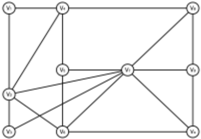
{v1, v3, v4, v5, v6, v8, v9, v10} according to Fix-out Reduction Rule 2. Then, v2 ≻ v1, so Vin = Vin ∪ v2. As a result, all vertices are added into Vin or Vout.
The time complexity of the Fix-I Reduction Rule 1, FixOut Reduction Rule 2, and the Fix-In Reduction Rule 3 are O(|E| × ∆), O(|E| × ∆), and O(|V | + |E|), respectively, where ∆ is the largest degree in G. These three reduction rules cover the all scenarios in which rules applied in EMDSP [Xiong and Xiao, 2024], which is the state-of-the-art exact algorithm for the MDS. Key differences between the above reduction rules and EMDSP reduce, along with their respective time complexity derivation procedures, are provided in the supplementary material. Despite the above reduction rules, we further propose another new reduction rule.
Fix-Out-Set Reduction Rule 4. For two vertices v1, v2 ∈ V , a vertex set VS′ ⊆ V \ Vout and |VS′ | > 1, if {v1, v2} △ VS′ , then
where CSet = {v′ ∈ VS′ \ N[Vin] | N[v′ ] ⊆ (VS′ ∪ Vout ∪ {v1, v2})}.
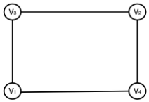
The time complexity of the above reduction rule is O(|V |2 ×∆2 ). The detailed derivation procedure is provided in the supplementary material. We also provide a small example to illustrate this reduction rule in Figure 2. Obviously, this square example cannot be reduced by the first three reduction rules. But it can be reduced by the Fix-Out-Set Reduction Rule 4 as follows: First, the Vin, Vout, and Vigore are initialized as ∅. Additionally, we can obtain {v1, v2} △ {v3, v4}, and CSet = {v3, v4}. After that, according to the Fix-Out-
Algorithm 1: DPRM
Input: An graph G = (V, E) Output: ⟨Vin, Vout⟩ 1 Vin := Vout := Vignore := ∅; 2 repeat 3 foreach v ∈ V Vin und \ Vignore do 4 if ∃v′ ∈ N(v) ∩ V Vin und \ Vignore, {v} ▶ {v′ } then 5 Vignore = Vignore ∪ {v}; 6 foreach v ∈ V \ Vout do 7 if ∃v′ ∈ N(v) ∩ (V \ (Vin ∪ Vout)), {v} △ {v′ } then 8 Vout = Vout ∪ {v′ }; 9 foreach v ∈ V \ V Vin und do 10 if ∃v′ ∈ N[v], N[v] \ Vout = {v′ } then 11 Vin := Vin ∪ {v′ }; 12 until no vertices are added into Vin, Vout and Vignore; 13 if V \ (Vin ∪ Vout)| <M then 14 apply Fix-out-Set Reduction Rule 4 thoroughly; 15 apply Fix-In-Set Reduction Rule 3 thoroughly; 16 else 17 sample N vertex pairs from V \ (Vin ∪ Vout); 18 apply Fix-out-Set Reduction Rule 4 for the above vertex pairs; 19 apply Fix-In-Set Reduction Rule 3 thoroughly; 20 return ⟨Vin, Vout⟩Set Reduction Rule 4, Vout = Vout ∪ {{v3, v4} \ N[v3]} ∪ {{v3, v4} \ N[v4]} = {v3, v4}. Then, we will get v1 ≻ v1, v2 ≻ v2. As a result, Vin = {v1, v2}.
3.3 The DPRMAlgorithm
We present the DPRM algorithm in Algorithm 1. The DPRM algorithm begins by initializing Vin, Vout and Vignore. Then, it entering a loop that sequentially applies the Fix-I Reduction Rule 1, Fix-Out Reduction Rule 2, and Fix-In Reduction Rule 3 (Lines 2-12). For each vertex v, we traverse each of its neighbors v′ and check whether v and v′ satisfy the conditions specified by the three reduction rules (Lines 4, 7, and 10). This loop continues until no vertices are added to Vin, Vout, and Vignore (Line 12).
Afterward, since Fix-Out-Set Reduction Rule 4 have a higher time complexity, we apply this reduction rule as follows: If the number of remaining vertices is less thanM after the reduction, we thoroughly apply the Fix-Out-Set Reduction Rule 4 and Fix-In Reduction Rule 3 (Lines 13-15). Otherwise, we randomly select N pairs of vertices and treat each of them as the {v1, v2} of the two reduction rules. Then we conduct these two reduction rules for the selected N vertex pairs (Lines 17-19). Based on our preliminary experiments, we set M as 1000 and N as 10000.
4 Two-Phase InitializationMethod
In this section, we first review previous initialization methods adopted by the local search algorithms for the MDS. Then, our two-phase initialization method is presented.
4.1 Previous InitializationMethods for MDS
The initialization procedure commonly used by previous local search algorithms for the MDS is typically a greedy approach, denoted as Initgreedy [Fan et al., 2019; Cai et al., 2020]. This method greedily adds vertices with the largest score to the candidate set until all the vertices are dominated. Furthermore, Zhu et al. [2024] integrate a perturbation process into Initgreedy, resulting in a perturbation initialization method denoted as Initperturb. In DmDS [Zhu et al., 2024], both Initgreedy and Initperturb are conducted, and the best initial solution obtained from these two methods is selected.
4.2 Two-Phase Initialization Procedure
The classic Initgreedy method adds the vertex with the largest score at each iteration. These high-score vertices are usually located in dense areas of the graph, which often leads to the neglect of vertices in sparse areas. In fact, how to dominate these vertices is critical to the initialization process. This is because vertices in sparse areas tend to dominate a small number of neighbors, meaning that a larger number of vertices is needed to dominate the same number of vertices in sparse areas compared to dense areas.
Different from previous methods, our initial solution prioritizes the addition of vertices that can dominate sparse areas. Specifically, we adopt k-shell decomposition [Kitsak et al., 2010] to partition the graph into different areas. There are several cluster sets CS = {V1, V2, . . . , Vn} in the k-shell decomposition, and each set Vi is associated with a shell value denoted as shell(Vi), where a higher shell(Vi) value indicates Vi is located in a denser area. At the beginning, CS is initialized as an empty set, then the k-shell algorithm iteratively removes a set of vertices from the graph. In the ith iteration, the minimum degree of all the vertices is recorded as dmin, and vertices with the degree value not higher than dmin are removed from the given graph and then they are stored in Vi until the degree value of all the remaining vertices is larger than dmin. Then, the set of removed vertices Vi is added to CS. After that, the shell value of the current vertex subset Vi ∈ CS is set to dmin, i.e., shell(Vi) = dmin. The shell decomposition process continues until all vertices have been removed from the graph. Its time complexity is O(|V |+|E|).
The complete two-phase initialization method is shown in Algorithm 2. At first, the algorithm proceeds with the k-shell decomposition procedure and stores all vertex subsets with a shell value less than del thre in the candidate set CSsp, where del thre is a parameter (Lines 1-2). The initial solution D is set to an empty set (Line 3). In the following, there are two phases, including the priority phase (Lines 4-9) and the greedy phase (Lines 10-12). In the first phase, if CSsp is not empty, the algorithm iteratively selects a vertex subset Vi with the smallest shell value, breaking ties randomly (Line 5). For each vertex vp ∈ Vj ∩ V D und , the algorithm selects an added vertex from N[vp] \ Vout with the largest score value,
Algorithm 2: Inittp
Input: A graph G = (V, E), fix-in set Vin, fix-out set Vout Output: An initial solution D 1 applying k-shell decomposition to obtain a cluster set CS; 2 CSsp := {Vi ∈ CS | shell(Vi) < del thre}; 3 D := Vin; 4 while CSsp ̸= ∅ do 5 select a vertex subset Vj with the minimum shell value; 6 foreach vp ∈ Vj ∩ V D und do 7 select a vertex vadd ∈ N[vp] \ Vout with the largest score value; 8 D := D ∪ {vadd}; 9 CSsp := CSsp \ {Vj}; 10 while V D und ̸= ∅ do 11 select a vertex vadd ∈ V \ Vout with the largest score value; 12 D :=D∪ {vadd}; 13 return D;and then adds it into D (Lines 7-8). The vertex subset Vi is removed from CSsp (Line 9). In the second phase, a vertex with the largest score value and outside the Vout is iteratively added until all the vertices are dominated (Lines 10-12). Finally, the algorithm returns an initial solution D (Line 13).
5 The NuMDS Algorithm
We present a novel multi-stage search mechanism, followed by introducing our proposed algorithm namely NuMDS.
5.1 Multi-Stage SearchMechanism
Previous local search algorithms for the MDS and MWDS have commonly employed a unified search approach throughout the entire search procedure [Chalupa, 2017; Fan et al., 2019; Cai et al., 2020; Chen et al., 2023]. However, this type of search pattern lacks the flexibility to adapt various search approaches based on the current search state. The local search usually faces two main challenges, including slow convergence speed during the early stages of the search and difficulty in escaping from local optima during the later stages of the search. To deal with these challenges, we propose a multi-stage local search mechanism that incorporates different search manners at different stages of the search. In the early stages of the search, we employ a greedy manner to accelerate the convergence speed of the search. If improving the quality of current solution becomes gradually challenging, we adopt two kinds of manners sequentially, including random and exploitation search manners.
During the local search, we use a variable unimprove to measure the current state of the search, which is defined as the number of consecutive steps during the local search where the best solution has not been improved. As the value of unimprove increases, it indicates that improving the quality of the current solution is pretty hard. Moreover, we define a hybrid scoring function to evaluate each vertex in the candidate solution D, formally expressed as follows: ∀v ∈ D, scorehybrid(v) = age(v) |score(v)|+1 , where the age value of vertex v is defined as the number of steps for which the vertex has not been operated (i.e., to be added or removed). This function considers both the diversification effect and the direct impact of operating a vertex in D. Its goal is to prioritize selecting vertices that have not been operated for a long period while simultaneously resulting in few undominated vertices.
The proposed mechanism modifies the vertex removal procedure of the local search to align with three search manners. Thus, how to define search manner is a key issue. We employ three variations of the best from multiple selections heuristic (BMS) [Cai, 2015] by adjusting the parameter settings to match the respective search manners. The BMS strategy works as follows, i.e., randomly sampling a certain amount of vertices and then selecting the best one among them. In the following, we give three search manners.
Greedy Search Manner. If unimprove < thre, the algorithm randomly samples t1 vertices from D \ Vout and removes the one with the smallest score value, breaking ties with the largest age value.
Random Search Manner. If thre ≤ unimprove < 2 × thre, the algorithm removes a random vertex from D \ Vout. Exploitation SearchManner. If unimprove ≥ 2×thre, the algorithm randomly samples t1 vertices from D \ Vout, and removes the one with the largest scorehybrid value, breaking ties randomly.
Where thre and t1 are two parameters. Note that the scorebased vertex removal procedure indicates a greedy manner, which limits the total number of undominated vertices. Regarding the transition to the second and third search manners, the algorithm gradually enhances the exploration capability of the search. As the value of unimprove increases, the search procedure naturally shifts its inclination from exploration to exploitation, i.e., from the random search manner to the exploitation search manner. Specifically, for the third search manner, removing vertices with the largest scorehybrid value can be beneficial for escaping from local optima.
5.2 Details of the NuMDS
The proposed algorithm NuMDS is presented in Algorithm 3. First, the DPRM is applied to generate the Vin and Vout, and unimprove is initialized as 0 (Lines 1-2). Subsequently, the proposed initialization method is employed to obtain an initial solution, which serves as the starting point of the following local search procedure (Line 3). In each iteration, the algorithm begins by checking whether the undominated vertex set V D und is empty. If so, the algorithm iteratively removes some redundant vertices (Lines 6-8). The best solution Dbest is updated by D and unimprove is reset to 0 (Line 9). Lastly, the algorithm utilizes the BMS heuristic to remove a vertex with the largest score value, resulting in an unfeasible candidate solution smaller than Dbest (Lines 10-11).
After that, the local search turns to begin a swap procedure, involving removing two vertices and adding two other vertices (Lines 13-22). Specifically, during the vertex removing procedure, the first removal vertex is selected using the BMS strategy to choose a vertex with the largest score value, whereas the second removal vertex is selected according to the proposed three search manners (Lines 13-17). During the
Algorithm 3: NuMDS
Input: A graph G = (V, E) Output: the best obtained solution Dbest 1 ⟨Vin, Vout⟩ :=DPRM(G); 2 unimprove := 0; 3 D :=Dbest := Inittp(G, Vin, Vout); 4 while elapsed time < cutoff do 5 if V D und = ∅ then 6 while there exist vertices in D whose score is 0 do 7 select a vertex v1 ∈ D \ Vin with score(v1) = 0; 8 D := D \ {v1}; 9 Dbest :=D and unimprove := 0; 10 select a vertex v2 ∈ D \ Vin with the largest score among t2 samples, breaking ties by the largest age; 11 D := D \ {v2}; 12 continue; 13 remove a vertex v1 ∈ D \ Vin with the largest score among t2 samples, breaking ties by the largest age value; 14 D :=D \ {v1}; 15 choose a search manner based on the unimprove value; 16 select a vertex v2 based on the corresponding manner; 17 D :=D \ {v2}; 18 select a vertex u1 ∈ V D und \ Vout with the largest score value, breaking ties by the largest age value; 19 D :=D∪ {u1}; 20 if V D und = ∅ then 21 select a vertex u2 ∈ V D und \ Vout with the largest score value, breaking ties by the largest age value; 22 D := D ∪ {u2}; 23 unimprove := unimprove +1; 24 return Dbest;| Parameter | Range | Final value |
|---|---|---|
| t1 t2 del thre | {5, 10, 15, 20} | 10 |
| {35, 40, 45, 50} | 45 | |
| thre | {4, 6, 8, 10} | 6 |
| {2000, 2500, 3000} | 2500 |
vertex adding procedure, if undominated vertices exist, two vertices with the largest score value are sequentially added (Lines 18-22). In case multiple vertices have the same score for these two procedures, ties are broken by favoring the vertex with the largest age value. At the end of each iteration, unimprove is increased by 1 (Line 23). The local search terminates when the current run time reaches the predefined cutoff time (Line 4). Finally, the best solution Dbest is returned (Line 24).
6 Experiments
We conduct extensive experiments to evaluate the performance of NuMDS. According to previous studies [Cai et al., 2020; Zhu et al., 2024], DmDS [Zhu et al., 2024] and FastDS [Cai et al., 2020] significantly outperform other heuristic algorithms for the MDS. Thus, we first select these two algorithms as our competitors. Besides, we compare NuMDS with the state-of-the-art MWDS solver DeepOptMWDS [Chen et al., 2023]. The source codes of all algorithms are kindly provided by the authors. All the algorithms are implemented in C++ and compiled by g++ with -O3 option. All experiments are conducted on Intel Xeon Gold 6238 CPU @ 2.10GHz with 256GB RAM under CentOS 7.9. For all comparative algorithms, we use the parameters specified in the corresponding literature. Note that the experiments in DmDS were conducted on a significantly more powerful CPU than ours. To achieve the results reported in the literature, we set the time limit to 1800 seconds. For each instance, all algorithms are executed 10 times with the random seeds from 1 to 10.
We collect all instances that have already been tested by DmDS [Zhu et al., 2024] and FastDS [Cai et al., 2020], comprising 4 standard benchmarks and 4 real-world benchmarks. The selected benchmarks are presented as follows.
UDG. This benchmark is widely used in many algorithms for the MDS [Hedar and Ismail, 2010b; Potluri and Singh, 2011; Cai et al., 2020; Zhu et al., 2024]. UDG comprises 12 families, and each family contains 10 instances.
T1. This benchmark consists 54 families, with each family containing 10 instances of the same size. Each instance has two weight functions [Romania, 2010] and we set the weight of each vertex to 1.
DIMACS. This benchmark is sourced from the Second DIMACS Implementation Challenge (1992-1993) 2 . It has been extensively tested in various significant combinatorial optimization problems, including 61 instances.
BHOSLIB. This benchmark is generated from RB model [Xu et al., 2007], containing 41 instances.
SNAP. The Stanford Large Network Dataset Collection comprises a collection of real-world graphs ranging from 104 vertices to 107 vertices in size.
DIMACS10. This benchmark is sourced from the 10th DIMACS Implementation Challenge (2010) 3 , containing many challenging instances.
Network Repository. The Network Data Repository [Rossi and Ahmed, 2015] is a comprehensive collection of real-world graphs gathered from various domains.
The standard benchmarks have 168 instances, including UDG, T1 and DIMACS and BHOSLIB, and the remaining benchmarks have 260 real-world instances. In total, we select 428 instances. In detail, for the instances selection of SNAP and DIMACS10, we follow the DmDS and FastDS [Cai et al., 2020; Zhu et al., 2024]. Only instances with a minimum of 30,000 vertices are chosen, resulting in a set of 53 instances. For the Network Repository, many previous studies for the MDS and MWDS select vertices with more than 105 and edges with more than 106 [Wang et al., 2018; Cai et al., 2020; Chen et al., 2023], resulting in 65 instances. In 2024, Zhu et al. [2024] add 142 additional instances from NDR to test the performance of DmDS. Consequently, we divided the instances in the Network Repository into two sets:
2 ftp://dimacs.rutgers.edu/pub/challenges
3 https://www.cc.gatech.edu/dimacs10/
| Benchmark | #ins | NuMDS #min(#avg) | DmDS min(#avg) | FastDS #min(#avg) | DeepOpt-MWDS #min(#avg) |
|---|---|---|---|---|---|
| UDG | 12 | 12(12) | 12(12) | 11(9) | 12(12) |
| T1 | 54 | 54(53) | 44(29) | 49(41) | 47(43) |
| DIMACS | 61 | 61(60) | 55(47) | 59(53) | 59(55) |
| BHOSLIB | 41 | 41(41) | 33(13) | 35(26) | 26(17) |
| DIMACS10 | 31 | 23(24) | 12(11) | 10(10) | 10(9) |
| SNAP | 22 | 20(20) | 14(11) | 13(11) | 16(13) |
| NDR1 | 65 | 62(61) | 37(31) | 32(27) | 26(22) |
| NDR2 | 142 | 137(117) | 58(70) | 51(44) | 45(42) |
| #total | 428 | 410(388) | 265(224) | 260(221) | 241(213) |
NDR1 and NDR2. NDR1 consists of the 65 instances tested by previous studies for the MDS, and NDR2 comprises the 142 additional instances added by DmDS.
We utilize the automatic configuration tool irace [L´opezIb´a˜nez et al., 2016] to tune the parameters. For the training set, we randomly selected 10% instances from each benchmark. The tuning process is given a budget of 4000 runs for the training set with a time budget of 1000 seconds per run. Table 1 presents the selected parameter values. For all competitors, we used the parameters from the relevant literature and optimized them for the newly added instances using the irace tool.
Despite using irace for parameter tuning, we manually analyze the parameter sensitivity of NuMDS as follows. Initially, we select 10% instances from each benchmark, resulting in a total of 41 instances. We vary t1 with values 5, 10, and 15, t2 with values 40, 45, and 50, and thre with values 2000, 2500, and 3000. In total, we tested 27 different parameter combinations. NuMDS is executed within a cutoff time of 1800 seconds using random seeds of 1 to 10. According to our experiments, under the optimal parameter settings, the best solution achieved is, on average, 0.0021% smaller than the best solutions obtained using other parameter combinations. Additionally, we selected del thre as 4 and 8. The initial solution achieved with del thre set to 6 is, on average, 0.0017% smaller than the initial solutions obtained with del thre set to 4 and 8. These results show that the performance our algorithm is not sensitive to the parameters.
6.1 Results on All the Benchmarks
Results on all the benchmarks are summarized in Table 2. We present the detailed results of NuMDS and all competitors in the supplementary material.
Results on standard and real-world benchmarks
For all standard benchmarks, NuMDS can find the best solution for all the instances. Specifically, NuMDS outperforms FastDS, DmDS, and DeepOpt-MWDS for 14, 24, and 24 instances. Furthermore, among 168 standard instances, it only fails to obtain the minimal average solution on only 2 instances, while FastDS, DmDS, and DeepOpt-MWDS fail to achieve the minimal average solution for 39, 67, and 41 instances. As for the real-world instances, NuMDS performs best on all the benchmarks. In detail, it obtains the 23 best solutions (out of 31 instances) on DIMACS10 benchmark,

| Benchmark | #ins | vs. Gurobi #bet(#wor) | vs. BIBLP #bet(#wor) |
|---|---|---|---|
| Standard | 168 | 73(1) | 72(1) |
| SNAP&DIMACS10 | 53 | 22(10) | 43(0) |
| NDR1 | 65 | 31 (4) | 62(0) |
| NDR2 | 142 | 86(6) | 113(0) |
| #total | 428 | 212(21) | 290(1) |
| Benchmark | #ins | vs. NuMDS1 #bet(#wor) | vs. NuMDS2 #bet(#wor) | vs. NuMDS3 #bet(#wor) | vs. NuMDS4 #bet(#wor) | vs. NuMDS5 #bet(#wor) | vs. NuMDS6 #bet(#wor) | vs. NuMDS7 #bet(#wor) |
|---|---|---|---|---|---|---|---|---|
| Standard | 168 | 0(0) | 0(0) | 0(0) | 6(0) | 0(0) | 0(0) | 8(0) |
| S&D | 53 | 20(8) | 19(2) | 13(6) | 17(5) | 19(3) | 12(6) | 13(0) |
| NDR1 | 65 | 25(3) | 13(3) | 15(8) | 23(5) | 18(3) | 16(8) | 21(2) |
| NDR2 | 142 | 80(12) | 45(12) | 44(21) | 83(3) | 64(7) | 61(7) | 66(4) |
| #total | 428 | 125(23) | 77(17) | 72(35) | 129(13) | 101(13) | 89(21) | 108(6) |
| Benchmark | Infe rules | RLNSV | RLNSV imp | EMDSP reduce | DPRM | |||||
|---|---|---|---|---|---|---|---|---|---|---|
| fix ratio | time | fix ratio | time | fix ratio | time | fix ratio | time | fix ratio | time | |
| Standard | 0.18% | <1 | 0.69% | <1 | 1.31% | <1 | 12.54% | <1 | 13.32% | <1 |
| SNAP&DIMACS10 | 21.82% | <0.1 | 32.67% | 1.04 | 47.81% | 1.94 | 56.15% | 20.03 | 68.47% | 6.11 |
| NDR1 | 29.07% | <0.1 | 36.75% | 4.29 | 62.98% | 18.3 | 67.94% | 22.68 | 72.83% | 30.27 |
| NDR2 | 12.53% | <0.1 | 16.10% | 8.77 | 27.36% | 8.22 | 32.74% | 278.10 | 53.41% | 39.64 |
| Benchmark | #ins | vs. FastDS #bet(#wor) | vs. DmDS bet(#wor) |
|---|---|---|---|
| Standard | 168 | 0(0) | 0(0) |
| SNAP&DIMACS10 | 53 | 24(6) | 19(3) |
| NDR1 | 65 | 25 (6) | 25(6) |
| NDR2 | 142 | 81(9) | 61(23) |
| #total | 428 | 130(21) | 105(32) |
20 best solutions (out of 22 instances) on SNAP benchmark, 62 best solutions (out of 65 instances) on NDR1 benchmark, 130 best solutions (out of 142 instances) on NDR2 benchmark. Every competitor fails to obtain over 50% best solutions among 260 real-world instances. Moreover, when NuMDS discards its training set in the parameter tuning procedure, it achieves 371 best solutions out of 387 instances, while DmDS, FastDS, and DeepOpt-MWDS achieve 242, 236, and 217 best solutions, respectively.
Run time analysis
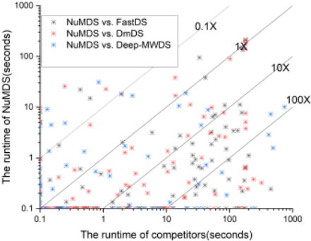
Then, we conduct a run time comparison between the NuMDS algorithm and three comparison algorithms, focusing on cases where both algorithms achieved the same best and average solution values for all instances. The instances where the run time of both NuMDS and the corresponding competitors is below 0.1 seconds are excluded from the analysis. As shown in Figure 3, the run time obtained by NuMDS is quite smaller than its competitors for the most instances.
Critical Difference Plots for All Algorithms
We use statistical analysis to evaluate the performance of the NuMDS algorithm and its competitors by presenting the difference of the best solutions obtained by each algorithm in Figure 4. First, we conduct the Friedman Test [Friedman,
1937] with the null hypothesis that the NuMDS algorithm performs equally to all the competitors. If the null hypothesis is rejected, we perform the Nemenyi post-hoc test for pairwise comparisons. The results are then presented using a critical difference diagram [Garcıa and Herrera, 2008]. A lower rank indicates better performance. If the difference between algorithms is not statistically significant at a significance level of 0.05, it indicates a connection between those algorithms. According to the critical difference plots, NuMDS consistently outperforms all the competitors.
6.2 Further Results with Exact Algorithms
In this part, we compare the NuMDS with the state-of-theart exact algorithms. According to the literature [Jiang and Zheng, 2023; Xiong and Xiao, 2024], the state-of-the-art algorithm for the MDS is BIBLP [Xiong and Xiao, 2024]. So we compare NuMDS with this algorithm. Moreover, we also compare NuMDS with one of the most powerful commercial mixed integer programming (MIP) solvers Gurobi [Gurobi Optimization, 2021]. The version used is 10.0.3.
Note that the Gurobi is conducted on the instances reduced by DPRM. The time limit of the two exact algorithms are set to 1800 seconds, and we compare them with NuMDS under the cutoff time of 1800 seconds and seed 1. We summary the compared results in Table 3. As shown in Table 3, NuMDS clearly outperforms the two algorithms.
6.3 Analysis on the Proposed Strategies
First, we evaluate the proposed strategies by comparing NuMDS with its seven alternative versions: (1) NuMDS1 replaces the DPRM with the Infe-rules; (2) NuMDS2 substitutes the DPRM with the RLNSV imp; (3) NuMDS3 substitutes the DPRM with the EMDSP reduce; (4) NuMDS4 eliminates the multi-stage mechanism and instead adopts the same second vertex selection method as DmDS [Zhu et al., 2024] and FastDS [Cai et al., 2020]. Specifically, in each iteration of the NuMDS, the second removal vertex is selected randomly. NuMDS5, NuMDS6, and NuMDS7, each removing one of the search modes: greedy search, random search, and exploitation search, respectively. Table 4 shows that both DPRM and the multi-stage mechanism are indispensable in the proposed NuMDS.
| Benchmark | #ins | Inittp #win(#time) | Initgreedy #win(#time) | Initperturb #win(#time) |
|---|---|---|---|---|
| realworld | 260 | 209(4.75) | 47(14.45) | 50(16.18) |
| Benchmark | #ins | Inittp #win(#time) | Initgreedy #win(#time) | Initperturb #win(#time) |
|---|---|---|---|---|
| realworld | 260 | 232(5.36) | 33(16.4) | 29(16.21) |
Then, we present the fix ratio and time consumption among DPRM, RLNSV [Alber et al., 2004], RLNSV imp [Alber et al., 2006], the inference rules used in FastDS [Cai et al., 2020] (referred to as Infe-rules), and the EMDSP reduce in Table 5. We don't present the comparison result of RLNPV and RLNPV imp due to their extremely long time consumption on real-world instances, making them unsuitable to be applied in local search algorithms. Specifically, both RLNPV and RLNPV imp have a time consumption exceeding 1800 seconds on 87% real-world instances.
Table 5 shows that the fix ratio achieved by the DPRM reduction method is consistently better than that of other reduction techniques, except when compared to the EMDSP reduce on standard instances. When compared to Infe rules, RLNSV, and RLNSV imp on real-world instances, DPRM significantly outperforms these algorithms in terms of fix ratio. Although the DPRMmethod has a longer time consumption than these algorithms, its run time remains within an acceptable range. Moreover, when we compare DPRM to EMDSP reduce on real-world instances, DPRM also shows an improvement on all benchmarks. Overall, DPRM demonstrates robust performance in both fix ratio and time consumption.
Subsequently, we investigate the impact of DPRM on the local search performance. We incorporate DPRM into FastDS and DmDS, resulting in FastDSDPRM and DmDSDPRM, and compare the best solutions obtained by these two algorithms with the best solution obtained by the original algorithms. The results are presented in Table 6. It is evident that DPRM greatly enhances the performance of FastDS and DmDS.
After that, we conduct experiments to evaluate the performance of two-phase initialization method. First, we compare Inittp with Initgreedy and Initperturb. Then, we don't use any reduction rules and directly evaluate the performance of the three initialization procedures. Note that the instances in the standard benchmark are significantly small, and the impact of the initial solution on the local search procedure can be omitted. Therefore, we only focus on the real-world benchmarks. As shown in Tables 7 and 8, Inittp outperforms previous initialization methods in terms of both initial solution quality and time consumption. It demonstrates the good performance regardless of whether the reduction process is employed. The reduced time consumption is a result of the vertex selection procedure in the priority phase, which only needs to transverse the neighbors of specific vertices, rather than traversing all vertices not in the candidate solution.
7 Conclusion
This paper proposes an efficient local search algorithm NuMDS for the MDS, which comprises three key ideas. First, a dominate propagation-based reduction method is presented to fix portion of vertices. Then, we develop an efficient twophase initialization method to start the search procedure from a good point. Finally, a multi-stage local search procedure is proposed, which adapts some suitable search manners. Extensive experimental results clearly demonstrate the effectiveness of NuMDS.
Acknowledgments
This work is supported by National Cryptologic Science Fund of China 2025NCSF02046, NSFC under Grant No. 61806050, the Fundamental Research Funds for the Central Universities 2412023YQ003, Jilin Science and Technology Department YDZJ202201ZYTS412.
@inproceedings{ijcai2025p997,
  title     = {NuMDS: An Efficient Local Search Algorithm for Minimum Dominating Set Problem},
  author    = {Sun, Rui and Liu, Zhaohui and Wang, Yiyuan and Xiao, Han and Li, Jiangnan and Chen, Jiejiang},
  booktitle = {Proceedings of the Thirty-Fourth International Joint Conference on
               Artificial Intelligence, {IJCAI-25}},
  publisher = {International Joint Conferences on Artificial Intelligence Organization},
  editor    = {James Kwok},
  pages     = {8966--8976},
  year      = {2025},
  month     = {8},
  note      = {Main Track},
  doi       = {10.24963/ijcai.2025/997},
  url       = {https://doi.org/10.24963/ijcai.2025/997},
}
TY - CPAPER TI - NuMDS: An Efficient Local Search Algorithm for Minimum Dominating Set Problem AU - Sun, Rui AU - Liu, Zhaohui AU - Wang, Yiyuan AU - Xiao, Han AU - Li, Jiangnan AU - Chen, Jiejiang T2 - Proceedings of the Thirty-Fourth International Joint Conference on Artificial Intelligence, IJCAI-25 PB - International Joint Conferences on Artificial Intelligence Organization PY - 2025 SP - 8966 EP - 8976 DO - 10.24963/ijcai.2025/997 UR - https://doi.org/10.24963/ijcai.2025/997 ER -Copied
Machine-readable versions of this paper, for tools and AI agents:
 Welcome
 Future Conferences
 AI Journal Division
 IJCAI Proceedings
 About IJCAI
 IJCAI Awards