
Bidirectional Search while Ensuring Meet-In-The-Middle via Effective and Efficient-to-Compute Termination Conditions
Proceedings of the Thirty-Fourth International Joint Conference on Artificial Intelligence. Main Track. Pages 8987-8995.
https://doi.org/10.24963/ijcai.2025/999
Keywords
- Search: S: Heuristic search
Abstract
In bidirectional heuristic search, the meeting-in-the-middle property (MMP) and the theory of must-expand pairs (MEP) have driven significant recent developments in search efficiency. However, these methodologies typically terminate the search based on minimal priority metrics in the forward and backward open lists, requiring exploration of all potentially better solutions and potentially incurring substantial computational burden. In this paper, we investigate the reasons that contribute to the potential inefficiency in MM , and introduce a tighter termination condition that enables earlier termination without exhaustive exploration while still ensuring both MMP and optimality. This results in a highly efficient bidirectional search algorithm.
Experimental comparisons demonstrate that our algorithm outperforms MM in terms of running time by at least two orders of magnitude and is on par or better compared to A*, highlighting its potential in a wide range of applications.
- [Alcázar et al., 2020] Vidal Alcázar, Patricia J. Riddle, and Mike Barley. A unifying view on individual bounds and heuristic inaccuracies in bidirectional search. In Associa- tion for the Advancement of Artificial Intelligence (AAAI), pages 2327-2334, 2020.
- [Arefin and Saha, 2010] Kazi Shamsul Arefin and Aloke Ku- mar Saha. A new approach of iterative deepening bi-directional heuristic front-to-front algorithm (IDB- HFFA). International Journal of Electrical and Computer Sciences, 10(2):13-21, 2010.
- [Auer and Kaindl, 2004] Andreas Auer and Hermann Kaindl. A case study of revisiting best-first vs. depth-first search. In European Conference on Artificial Intelligence (ECAI), volume 16, page 141, 2004.
- [Barker and Korf, 2015] Joseph Barker and Richard Korf. Limitations of front-to-end bidirectional heuristic search. In Association for the Advancement of Artificial Intelli- gence (AAAI), volume 29, pages 1086-1092, 2015.
- [Chen et al., 2017] Jingwei Chen, Robert C. Holte, Sandra Zilles, and Nathan R. Sturtevant. Front-to-end bidirec- tional heuristic search with near-optimal node expansions. In International Joint Conferences on Artificial Intelli- gence (IJCAI), pages 489-495, 2017. IJCAI
- [Eckerle et al., 2017] Jürgen Eckerle, Jingwei Chen, Nathan Sturtevant, Sandra Zilles, and Robert Holte. Sufficient conditions for node expansion in bidirectional heuristic search. In International Conference on Automated Plan- ning and Scheduling (ICAPS), volume 27, pages 79-87, 2017.
- [Felner et al., 2010] Ariel Felner, Carsten Moldenhauer, Nathan Sturtevant, and Jonathan Schaeffer. Single-frontier bidirectional search. In Association for the Advancement of Artificial Intelligence (AAAI), volume 24, pages 59-64, 2010.
- [Hart et al., 1968] Peter E Hart, Nils J Nilsson, and Bertram Raphael. A formal basis for the heuristic determination of minimum cost paths. IEEE transactions on Systems Sci- ence and Cybernetics, 4(2):100-107, 1968.
- [Helmert, 2010] Malte Helmert. Landmark heuristics for the pancake problem. In Symposium on Combinatorial Search (socs), volume 1, pages 109-110, 2010.
- [Holte et al., 2016] Robert C. Holte, Ariel Felner, Guni Sharon, and Nathan R. Sturtevant. Bidirectional search that is guaranteed to meet in the middle. In Association for the Advancement of Artificial Intelligence (AAAI), pages 3411-3417, 2016.
- [Holte et al., 2017] Robert C. Holte, Ariel Felner, Guni Sharon, Nathan R. Sturtevant, and Jingwei Chen. MM: A bidirectional search algorithm that is guaranteed to meet in the middle. Artificial Intelligence, 252:232-266, 2017.
- [Hu and Speck, 2022] Kilian Hu and David Speck. On bidi- rectional heuristic search in classical planning: An analy- sis of bae. In Symposium on Combinatorial Search (socs), volume 15, pages 91-99, 2022.
- [Kaindl and Kainz, 1997] Hermann Kaindl and Gerhard Kainz. Bidirectional heuristic search reconsidered. Jour- nal of Artificial Intelligence Research, 7:283-317, 1997.
- [Nicholson, 1966] T Alastair J Nicholson. Finding the short- est route between two points in a network. The computer journal, 9(3):275-280, 1966.
- [Pearl and Korf, 1987] Judea Pearl and Richard E Korf. Search techniques. Annual Review of Computer Science, 2(1):451-467, 1987.
- [Pearl, 1984] Judea Pearl, editor. Heuristics: Intelli- gent Search Strategies for Computer Problem Solving.
- [Russell and Norvig, 2020] Stuart J Russell and Peter Norvig. Artificial intelligence: a modern approach. Pearson, 2020.
- [Sadhukhan, 2012] Samir K Sadhukhan. A new approach to bidirectional heuristic search using error functions. In In- ternational Conference on Intelligent Infrastructure, 2012.
- [Sewell and Jacobson, 2021] Edward C Sewell and Shel- don H Jacobson. Dynamically improved bounds bidirec- tional search. Artificial Intelligence, 291:103405, 2021.
- [Shaham et al., 2017] Eshed Shaham, Ariel Felner, Jingwei Chen, and Nathan R. Sturtevant. The minimal set of states that must be expanded in a front-to-end bidirectional search. In Symposium on Combinatorial Search (socs), pages 82-90, 2017.
- [Shaham et al., 2018] Eshed Shaham, Ariel Felner, Nathan R. Sturtevant, and Jeffrey S. Rosenschein. Minimizing node expansions in bidirectional search with consistent heuristics. In Symposium on Combinatorial Search (socs), pages 81-89, 2018.
- [Shperberg et al., 2019a] Shahaf S. Shperberg, Ariel Felner, Solomon Eyal Shimony, Nathan R. Sturtevant, and Avi Hayoun. Improving bidirectional heuristic search by bounds propagation. In Symposium on Combinatorial Search (socs), pages 106-114, 2019.
- [Shperberg et al., 2019b] Shahaf S. Shperberg, Ariel Felner, Nathan R. Sturtevant, Solomon Eyal Shimony, and Avi Hayoun. Enriching non-parametric bidirectional search al- gorithms. In Association for the Advancement of Artificial Intelligence (AAAI), pages 2379-2386, 2019.
- [Siag et al., 2023] Lior Siag, Shahaf S. Shperberg, Ariel Fel- ner, and Nathan R. Sturtevant. Front-to-end bidirectional heuristic search with consistent heuristics: Enumerating and evaluating algorithms and bounds. In International Joint Conferences on Artificial Intelligence (IJCAI), pages 5631-5638, 2023. IJCAI
- [Sint and de Champeaux, 1977] Lenie Sint and Dennis de Champeaux. An improved bidirectional heuristic search algorithm. Journal of the ACM, 24(2):177-191, 1977.
- [Sturtevant and Felner, 2018] Nathan Sturtevant and Ariel Felner. A brief history and recent achievements in bidirec- tional search. In Association for the Advancement of Ar- tificial Intelligence (AAAI), volume 32, pages 8000-8006, 2018.
- [Sturtevant et al., 2020] Nathan R. Sturtevant, Shahaf S. Sh- perberg, Ariel Felner, and Jingwei Chen. Predicting the effectiveness of bidirectional heuristic search. In Interna- tional Conference on Automated Planning and Scheduling (ICAPS), pages 281-290, 2020.
- [Sturtevant, 2012] Nathan R Sturtevant. Benchmarks for grid-based pathfinding. IEEE Transactions on Computa- tional Intelligence and AI in Games, 4(2):144-148, 2012.
- [Uras and Koenig, 2015] Tansel Uras and Sven Koenig. An empirical comparison of any-angle path-planning algo- rithms. In Symposium on Combinatorial Search (socs), volume 6, pages 206-210, 2015.
- [Wang et al., 2025] Yi Wang, Eyal Weiss, Bingxian Mu, and Oren Salzman. Supplementary material for "meet-in- the-middle with early and efficient termination". https:// github.com/yi213-robotic/MEET, 2025. Accessed: 2025- 09-01. Link
References were extracted automatically from the PDF and may contain errors.
Full text extracted automatically from the PDF; figures, tables and equations may differ. The PDF is the version of record.
1 Introduction and RelatedWork
Search is a fundamental task in AI and robotics in which, in its simplest form, we wish to compute a minimal-cost path on a given graph between given start and goal vertices [Russell and Norvig, 2020]. Heuristics, which estimate the cost between states, allow to improve planner efficiency by focusing search efforts to smaller portions of the search space [Pearl, 1984]. Unidirectional heuristic search (Uni-HS) algorithms, such as A* [Hart et al., 1968], exemplify this principle by expanding the search from the start state to the goal.
Bidirectional search algorithms compute a solution by conducting two separate searches simultaneously: a forward search from the start, and a backward search from the goal [Nicholson, 1966]. In theory, a bidirectional search is capable of reducing the number of expanded states exponentially due to the search proceeding only to half the depth of the solution path [Nicholson, 1966; Pearl and Korf, 1987]. This theoretical efficiency renders bidirectional heuristic search (Bi-HS) a promising algorithmic approach. However, orchestrating the meeting of the forward and backward searches presents a significant challenge using heuristics (e.g., [Sint and de Champeaux, 1977; Kaindl and Kainz, 1997; Auer and Kaindl, 2004; Felner et al., 2010; Arefin and Saha, 2010; Barker and Korf, 2015; Siag et al., 2023]).
Arguably, there have been two conceptual breakthroughs in the field in the last decade [Sturtevant and Felner, 2018]: The first was the introduction of the meeting-in-the-middle propriety (MMP), which guarantees finding an optimal solution while also ensuring that each expanded state has a cost that is less than or equal to half of the cost of an optimal solution [Holte et al., 2016]. The second, which is an extension and generalization of the first, was a new theory of must expand pairs (MEP) for Bi-HS [Eckerle et al., 2017] which characterizes the set of forward and backward node pairs that must be expanded to guarantee solution optimality. Indeed, the majority of work in Bi-HS has been devoted to developing approaches that use these two concepts within Bi-HS algorithms in a computationally efficient manner.
Thus far, MM and its variants [Holte et al., 2017] did not achieve competitive running times when compared to the state-of-the-art in Uni-Hs and Bi-HS. In contrast, using the theory of MEP, many highly efficient, though arguably more complex, Bi-HS algorithms were suggested (e.g., [Shaham et al., 2017; Chen et al., 2017; Shaham et al., 2018; Shperberg et al., 2019a; Shperberg et al., 2019b; Sturtevant et al., 2020; Alc´azar et al., 2020]). When the heuristic used is known to be consistent 1 , the efficiency of these algorithms may be improved. Siag et al. (2023) presented an algorithmic framework unifying many of these algorithms. This also resulted in slight improvements to existing Bi-HS algorithms such as BAE* [Sadhukhan, 2012; Sewell and Jacobson, 2021]. As a general guideline, Siag et al. (2023) suggest that BAE* should be the default algorithm to use for the consistency case, as it strikes a good balance between node expansions and runtime across different domains and heuristics. Consequently, we use BAE* as a baseline.
In this paper, we revisit the MM-family of algorithms and study the reason to their practical inefficiency. We claim that this can be attributed to the termination condition (TC) used to decide when to stop MM's search. We suggest a tighter TC that preserves the theoretical properties of MM while being highly efficient to compute: In contrast to the TC employed by MM, our new TC does not require computing the minimal cost-to-come among all states in the forward and backward search. This allows (i) to perform state culling (i.e., to remove states that cannot be part of an optimal solution); and (ii) to efficiently test if the TC holds without the need to iterate over all states in the forward and backward search queues.
1 A heuristic function is said to be consistent if its value is always less than or equal to the estimated distance from any neighboring vertex to the goal, plus the cost of reaching that neighbor.
Meet-in-the-middle with Early and Efficient Termination (MEET) incorporates this new TC into an efficient Bi-HS algorithm that satisfies the MMP and is guaranteed to compute optimal solutions (i.e., it retains the same theoretical guarantees as MM). In contrast to conventional heuristic search algorithms, such as A*, which use a predefined admissible heuristic, MEET improves heuristic values on-the-fly, in a similiar fashion to MM, which increases its efficiency. Unlike Bi-HS algorithms that build on MEP theory, MEET halts the search by relying on cost metrics of a meeting state. Compared to BAE*, MEET achieves optimality without relying on the expansion of a meeting state that intersects on both search trees and lies on an optimal solution. Additionally, MEET is the first algorithm to address the open question of whether Bi-HS can terminate early while still ensuring optimality and MMP.
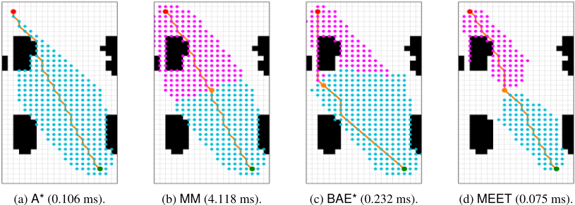
In this paper, we focus on the arguably simple MM-family of algorithms that do not require much of the advanced algorithmic building blocks developed using the general MEP theory. However, as we will see in the experimental results (Sec. 5), MEET is competitive and often outperforms stateof-the-art Bi-HS algorithms such as BAE*. To illustrate this, we visualize in Fig. 1 the states expanded by A*, MM, BAE*, and MEET in an instance on the grid map brc203 [Sturtevant, 2012], where MEET outperforms the other algorithms both in terms of the number of nodes expanded and the running time.
2 ProblemDefinitions and Notations
Let G = (S,E, c) be a weighted graph, where S is a set of states, E ⊆ S × S is a set of edges connecting states, and c : E → R≥ε is a cost function over the edges (i.e., we assume that the minimal edge cost is ε for some ε > 0). For a state s, we define the neighbors of s, denoted as nbr(s) to be all states that share an edge with s. Namely, nbr(s) := {s′ |(s, s′ ) ∈ E}. A path π = ⟨s0, . . . , sk⟩ is a sequence of states such that ∀i, si ∈ S and (si, si+1) ∈ E, where si is called the parent of si+1, and si+1 is called the child of si. We denote the parent of a state s in a path as prt(s). The cost of a path c(π) is defined as the sum of edge costs, i.e., c(π) := ∑i c(si, si+1). Given start and goal states sstart, sgoal ∈ S, a path connecting sstart to sgoal is also called a solution. A solution whose cost is minimal is called an optimal solution.
A Bi-HS algorithm simultaneously performs a search from sstart to sgoal (forward) and from sgoal to sstart (backward) until the searches meet at a state that lies on an optimal solution. We use subscripts 'F' and 'B' to denote the forward and backward search directions, respectively. For brevity, we primarily concentrate on the forward search direction, as the backward search (notations, definitions, analyses, etc.) is symmetrical and will be referenced only when specifically stated. When referring to an arbitrary direction D ∈ {F, B}, we denote its opposite by ¯D.
We denote by Π∗ and C ∗ the set of all optimal solutions and their cost. Given a state s we denote gF(s) the estimated cost to reach s from sstart as currently computed by the forward search. Furthermore, we define h∗F (s) to be the minimal cost among all paths connecting s to sgoal and assume that we are provided a heuristic function hF(s) that estimates h∗F (s). We say that hF is admissible if ∀ s ∈ S, hF(s) ≤ h∗F (s) and call hF static if it never changes its values during the search. Throughout this work, we assume that all static heuristics are admissible. Finally, we set fF(s) := gF(s) + hF(s).
As common in best-first heuristic search, all algorithms utilize OPENF, a priority queue that stores states generated in the forward search but not expanded (i.e., states with gF (s) < ∞), ordered by their fF-value. Similarly, CLOSEDF is a set of all states that have been expanded in the forward search.
We use πcurr and Ccurr to denote the current-best path and its cost as produced by a search algorithm at any given point in time. When an algorithm starts, πcurr is undefined and Ccurr = ∞. If it is guaranteed that πcurr ∈ Π∗ and Ccurr = C ∗ upon termination, then the algorithm is said to be optimal.
We use fmin-F and gmin-F to denote the minimal f-value and g-value among all states in OPENF, respectively. For OPENB we define fmin-B and gmin-B, analogously. Additionally, we set fmin := min (fmin-F, fmin-B) and gmin := min (gmin-F, gmin-B). Finally, with a slight abuse of notation, we set gmin(s) := min(gF(s), gB(s)).
We say that a state s ∈ S is an intersecting state if s ∈ OPENF ∩ OPENB. We denote by Icurr the set of all intersecting states that lie on paths with a cost equal to Ccurr. For the intersecting states, we set
Namely, Ib is an intersecting state that lies on a solution with Ccurr and has the minimal g-value among such states. We call Ib the current-best intersecting state. When the search ends with Ccurr = C ∗ , Ib serves as a meeting state, smeet.
Definition 1 (Meet-in-the-middle property [Holte et al., 2017]). ABi-HS algorithm satisfiesmeet-in-the-middle property (MMP) if it only expands states s with gD(s) ≤ C ∗ /2.
We say that a Bi-HS algorithm is MM-optimal if it is ensured to (i) return an optimal solution and to (ii) satisfy MMP.
3 Algorithmic Background
3.1 Algorithmic Framework
We start by outlining an algorithmic framework for an MMoptimal Bi-HS algorithm to standardize the core operations (Alg. 1). These key operations include state priority, state selection for expansion, state culling (or pruning), and TCs.
- State priority: A function that dictates how states are stored in the priority queues based on the estimated path cost in each search direction (Lines 1, 3 and 14).
- State selection for expansion: An operation that selects a state for expansion from the queues of both search directions. In a best-first approach, the selection should follow a priority function, which could be identical to the state priority, but not necessarily (Line 3).
- State pruning: A function that tests if discarding a state does not compromise MM-optimality (Line 12).
- Termination conditions: A termination criterion that allows the search to stop once no further expansion can improve Ccurr, ensuring MM-optimality, (Line 4).
3.2 Challenges in Bidirectional Heuristic Search
Unlike in Uni-HS, where the search termination is tied to a singular, clearly defined goal state, in Bi-HS the state in which the search should terminate, i.e., a meeting state, is implicitly defined. This raises a challenge: There is no guarantee of optimality when the forward and backward search fronts meet (i.e., when a solution is found). Thus, verifying
Input: G = (S, E, c), sstart, sgoal Output: Solution π 1 Insert sstart into OPENF and sgoal into OPENB using priority function 2 while both OPENF and OPENB are not empty do 3 Select s ∈ OPENF ∪ OPENB with min priority function 4 if ToTerminate then 5 return ReconstructPath 6 if s ∈ OPENF then 7 Remove s from OPENF 8 Add s to CLOSEDF 9 foreach s′ ∈ nbr(s) do 10 if s can't improve gF(s′ ) then 11 continue 12 if ToPrune(s′ ) then 13 continue 14 Insert s′ into OPENF using priority function 15 else 16 Analogous operation for the backward search 17 return ∅that a solution is optimal might incur unnecessary expansions if the TC is not tight. Conversely, tighter TCs can be computationally expensive to evaluate, and earlier termination poses a high risk of compromising optimality.
Indeed, significant research efforts were taken to derive effective TCs that ensure solution optimality in Bi-HS. This culminated in the work by Siag et al. (2023) who introduced a set of 17 search bounds (which included bounds from previous works) that can be used for determining optimality. Notably, utilizing combinations of them for obtaining a tighter TC introduces non-trivial computational overhead.
3.3 Meet-In-The-Middle (MM)
To obtain MMP, MM uses the following priority function when inserting a state s into OPENF where states are prioritized from low to high:
The ordering in OPENB is defined analogously. To understand the intuition behind this priority function, recall that to maintain MMP, an algorithm should only expand a state s if gF(s) ≤ C ∗ /2, identical to the condition 2gF(s) ≤ C ∗ . In addition, to ensure optimality, a state s should be expanded if fF(s) ≤ C ∗ , indicating it may lie on an optimal path.
Unfortunately, when a heuristic fails to accurately estimate the cost to reach the goal, then a state s with gF(s) > C ∗ /2 may have fF (s) < C ∗ , thereby violating MMP. This happens when gF(s) > hF(s). In this case, we say that h is a weak heuristic [Barker and Korf, 2015], and this may cause MM to expand states that can not be part of an optimal solution.
As a termination condition, MM halts the search once
Here, Cpr represents the minimum priority on both search fronts. Holte et al. [2017] show that each of the last three terms is a lower bound on the cost of any solution that might be found by continuing to search.
Importantly, this TC requires access to gmin and fmin from both OPEN lists at each iteration. Since MM does not sort its lists by g- or f-values (rather by prF defined above), each iteration in MM needs to iterate over all members of each OPEN list to obtain gmin and fmin. This comes with a significant computational overhead due to the exponential growth in the number of generated states as the search progresses. Consequently, a TC that can be computed efficiently, rather than with complexity O(|OPENF |+|OPENB|), could dramatically speed up the search process.
Finally, MM does not prune any states.
4 Meet-in-the-middle with Early and Efficient Termination (MEET)
In this section, we introduce MEET, our Bi-HS algorithm, which follows the structure as detailed in Alg. 1 and Sec. 3.1.
4.1 AlgorithmDescription
State Priority
Similar to MM, MEET defines the priority of a state s in OPEND according to its fD-value. However, the heuristic used is not the static heuristic hD but an updated one which we denote by ˜hD. Specifically, and with slight abuse of notation, fD(s) := gD(s) + ˜hD(s) where ˜hD(s) is initialized to be hD(s). In case s /∈ CLOSED ¯D ∪ {OPEN ¯D} and gD(s) > hD(s), ˜hD(s) is updated to be gD(s). Otherwise, if s ∈ OPEN ¯D, ˜hD(s) is set to be g ¯D(s). Note that for the simplicity of the presentation we make a slight abuse of notation and use the notation f rather than define a new notation for f with ˜h. Hence, whenever we describe MEET or results related to it, consider that f is used with ˜h.
State Selection for Expansions
Similar to MM, MEET selects the state whose priority equals fmin.
State Pruning
Before generating a new state s in direction D ∈ {F, B}, MEET tests whether
If so, s is discarded.
Termination Condition
MEET makes use of four termination conditions and terminates if one of them holds. When describing the termination conditions, we assume that a solution has been found (namely, C ∗ ≤ Ccurr) and that H ∈ {F, B} is the direction for which Ib has a larger g-value (i.e., gD(Ib) > g ¯D(Ib)). prtH(Ib) denote the parent of Ib in H direction. Furthermore, we denote s to be the state chosen for expansion (i.e., fD(s) = fmin) and s′ ∈ nbr(s) to be a neighbor that is generated in the expansion of s with minimal fD-value. Finally, we denote t as the state with fD (t) = fmin-D (i.e., the state with the minimal f-value in the opposite search direction).
MEET terminates if one of the following conditions holds:
Intuitively, TC1, also used by MM, indicates that no further expansion can improve the current best solution.
TC2 triggers if the lowest-priority states in both OPEN lists are too far apart, namely if the sum of their g-values plus the minimal edge cost exceeds Ccurr, so no further expansions can improve it, and thus the search can terminate early.
MEET has two more termination conditions (TC3 and TC4), for which we require further notation: We denote S(Ib, s) to be the set of states generated after Ib has been found (i.e., generated by both search directions) but before s was expanded. Note that S(Ib, s) may be empty. We now introduce an auxiliary precondition that needs to hold before using TC3 and TC4.
For the specific case where S(Ib, s) is empty, we define that PC1 does not hold. If PC1 holds, MEET terminates if one of the following conditions hold:
TC3 captures the intuition that if Ccurr is not yet optimal, then before expanding any child s′ of s with the minimal fvalue, there must already exist a newly generated ˜ s such that f{D, ¯D}(˜ s) ≤ 2gH(Ib). In other words, if no such ˜ s exists, and TC3 holds, then no further expansions can improve Ccurr and the search can stop early.
The logic and intuition of TC4 are similar to those of TC3. The two key differences in TC4 are that (1) f{D, ¯D}(˜ s) < Ccurr, and (2) it is applied when gD(Ib) ≤ g ¯D(Ib).
It is noteworthy that in all termination conditions, we do not need to compute the minimal g-value in OPENF and OPENB as in MM. In contrast, we rely on the readily available g and ˜h values that can be computed in constant time (e.g., of the best intersecting state and its parent). This is demonstrated in TC2 which is similar to the condition gmin-F +gmin-B +ε used by MM but is much cheaper to compute from a computational point of view.
4.2 Theoretic Properties and Guarantees
We now prove the correctness of MEET. We start by assuming the existence of an optimal solution with the length C ∗ going through a meeting state smeet, following C ∗ = gF(smeet)+gB(smeet). For all our proofs in this section, we set Sg>hD := {s | gD(s) > hD(s)}. Furthermore, we prove all lemmas for the forward direction, where the backward direction is analogous. We first prove that MEET satisfies MMP during expansions.
Lemma 1. MEET never expands a state s with gD(s) > C∗ 2 .
Proof. Assume, for contradiction, that MEET expands s with gD(s) > C∗ 2 . When s is generated, MEET sets ˜hD(s)
to either hD(s), gD(s), or g ¯D(s). As a result, fD(s) = gD(s) + ˜hD(s) ≥ gD(s) + gD(s) > C ∗ . Since MEET expands the states in a monotonically non-decreasing order of priority and fD(s) = fmin, it implies that all nodes with priority ≤ C ∗ have been expanded. As a result, MEET must already have found the optimal solution and such solution has been recorded, which means Ccurr = C ∗ . This contradicts the fact that s is selected for expansion only when fD(s) < Ccurr. Thus, MEET satisfies MMP.
We now prove that ˜h is an admissible heuristic for every state that is expanded.
Lemma 2. When MEET expands a state s, then ˜hD(s) ≤ h∗D (s) holds.
Proof. By Lemma 1, when s is selected for expansion, we directly have fD(s) = gD(s) + ˜hD(s) ≤ C ∗ . Thus, it provides
According to [Pearl, 1984], g∗D (s) ≤ gD(s) holds once fD(s) ≤ C ∗ . Moreover, for any s, we also have f ∗D (s) = g∗D (s) + h∗D (s) ≥ C ∗ . Substituting g∗D (s) ≤ gD(s) gives
We continue to examine each stopping condition individually to ensure optimality.
Lemma 3. If TC1 holds, MEET returns with C ∗ = Ccurr.
Proof. Since states are ordered according to their f-value from low to high, and due to ˜hF(s) being admissible when s is expanded (Lemma 2), once TC1 is met, we are guaranteed that no solution with an f-value lower than Ccurr exists.
Lemma 4. If TC2 holds, MEET returns with C ∗ = Ccurr.
Proof. We first prove that gD(s) + gD (t) + ε > Ccurr implies both 2(gD(s)+ε) > Ccurr and 2(gD (t)+ε) > Ccurr. We proceed by contradiction. Suppose 2(gD(s) + ε) ≤ Ccurr, equivalent to gD(s) + ε ≤ Ccurr 2 . Then, it follows Ccurr - gD(s) ≥ Ccurr 2 + ε. Since gD(s) + gD (t) + ε > Ccurr, we have gD (t)+ε > Ccurr -gD(s). Substituting the previous inequality, we obtain gD (t) + ε > Ccurr 2 +ε, indicating gD (t) > Ccurr 2 , which contradicts the fact that gD (t) < Ccurr 2 . By symmetry, assuming 2(gD (t) + ε) ≤ Ccurr similarly leads to a contradiction. Since Ccurr > C ∗ and gD(Ib) ≤ g ¯D(Ib), it implies that fD(si) < Ccurr must hold in at least one direction before finding C ∗ , contradicting the fact that 2(gD(s) + ε) > Ccurr and 2(gD (t) + ε) > Ccurr. Thus, Ccurr = C ∗ .
Lemma 5. If TC3 holds, MEET returns with C ∗ = Ccurr. If Ccurr > C ∗ , then the expansion of s, which occurs after Ib is found, will not have a child s′ such that gD(s′ ) = gD(s) + ε and gD(s′ ) > gH(Ib).
Proof. TC3 requires that when Ib appears in D, 2gD(Ib) > Ccurr and implies that any s′ in {D, ¯D} satisfies f{D, ¯D}(s′ ) > 2gD(Ib) after expanding prtD (Ib). By contradiction, since Ccurr > C ∗ , the search will eventually generate a state ˜ s with f{D, ¯D}(˜ s) < Ccurr < 2gD(Ib) before reaching Ccurr = C ∗ . Consequently, prt{D, ¯D} (˜ s) must have been expanded before s, contradicting TC3.
Lemma 6. If TC4 holds, MEET returns with C ∗ = Ccurr. If Ccurr > C ∗ , then the expansion of s, which occurs immediately after Ib is found, will not have a child s′ such that gD(s′ ) = gD(s) + ε and fD(s′ ) ≥ Ccurr.
Proof. The proof of Lemma 6 is similar to the proof of Lemma 5.
Theorem 1. MEET returns an optimal solution, if it exists.
Proof. By Lemmas 3-6, we establish that when either TC1, TC2, TC3 or TC4 hold it necessarily implies that C ∗ = Ccurr. Thus, MEET only terminates the search when an optimal solution is found. Furthermore, if a solution exists, then TC1 must hold at some point in the search, unless the search is terminated beforehand by one of the other termination conditions. Namely, MEET necessarily returns the optimal solution if a solution exists.
5 Experiments
In this section we compare MEET with A*, MM and BAE*, where the latter was chosen as a representative of the nonMM family of Bi-HS algorithms that provides state-of-the-art performance [Alc´azar et al., 2020]. 2 Additionally, we conducted an ablation study for MEET to separately assess the impact of using the ˜h heuristic instead of the static h heuristic and the impact of the pruning mechanism.
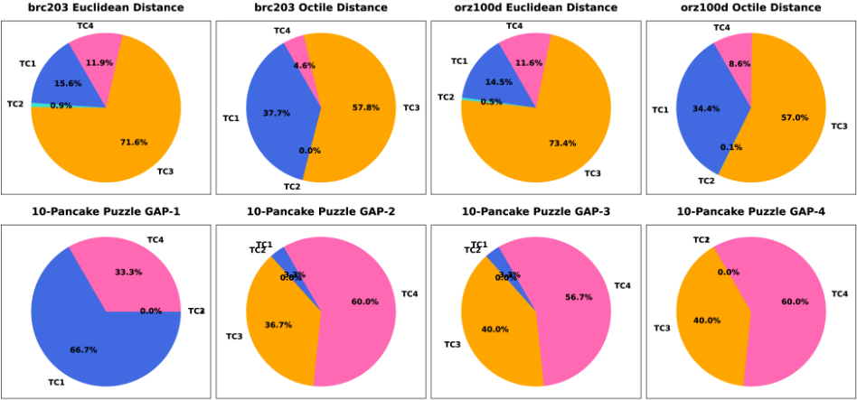
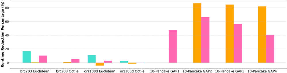
We ran experiments on two distinct domains: grid maps and 10-Pancake puzzles with all algorithms implemented in C++ on a desktop with 16GB RAM and an Intel i7 CPU running Ubuntu 20.04. The implementations of A*, MM, and BAE* were adapted from the source code of [Uras and Koenig, 2015], [Holte et al., 2017], and [Hu and Speck, 2022], respectively. Table 1 displays summarized experimental results for runtime statistics, while Fig. 2, 3, and 4 illustrate, respectively, the distributions of each triggered TC, the average percentages of runtime reduction achieved by each triggered TC vs. the baseline TC1, and detailed time distributions. The code implementation and additional results, including details on state expansions and reduction percentages, can be found in the supplementary material [Wang et al., 2025].
2 We also ran A* in the backward direction and MMe (a variant of MM with a different state priority function [Holte et al., 2017]), but these yielded very similar results to forward A* and MM, respectively, and were thus omitted.
| Domain | Heuristic | A* | MM | BAE* | MEET |
|---|---|---|---|---|---|
| brc203 | Euclidean Distance | 1.4 (0.42, 2.4) | 216 (52, 366) | 3.9 (1.3, 6.1) | 2.2 (0.65, 3.3) |
| Octile Distance | 1.6 (0.36, 3.1) | 406 (82, 879) | 4.3 (1.3, 6.5) | 2.4 (0.65, 3.8) | |
| orz100d | Euclidean Distance | 8.5 (1.8, 14.5) | 3.467×10³ (588, 6.411×10³ ) | 23.8 (5.2, 34.3) | 13.4 (2.7, 22.1) |
| Octile Distance | 9.2 (1.4, 16.5) | 5.214×10³ (864, 11.339×10³ ) | 25 (4.6, 37.2) | 14.7 (2.4, 24.5) | |
| 10-Pancake puzzle | GAP-1 | 0.31 (0.08, 0.75) | 7.1 (1.5, 22.3) | 0.46 (0.2, 1.5) | 0.48 (0.14, 0.74) |
| GAP-2 | 5.6 (3.6, 17.9) | 447 (110, 2.275×10³ ) | 1.3 (0.74, 3.1) | 1.0 (0.45, 2.1) | |
| GAP-3 | 81 (45.8, 291) | 12.189×10³ (403, 27.420×10³ ) | 8.2 (3.0, 24.8) | 3.9 (2.2, 11.1) | |
| GAP-4 | 510 (224, 1.605×10³ ) | 36.1326×10³ (529, 40.419×10³ ) | 26.1 (13.7, 78.8) | 6.5 (3.8, 32.5) |
5.1 GridMaps
We evaluate each algorithm on two grid maps from the MovingAI benchmark repository [Sturtevant, 2012], both originating from Dragon Age: Origins (DAO). These maps feature traversable regions that vary significantly across instances, providing substantial variability and ensuring a thorough evaluation of each algorithm's performance. An agent can move in an 8-way movement, and all evaluations use the Octile and Euclidean distance heuristics. The first map, brc203d (274 × 391), has 1290 instances, following [Holte et al., 2017]. The second map, orz100d (412 × 395), contains 2420 instances, and is considered relatively challenging, as the heuristics are often less informative on this map.
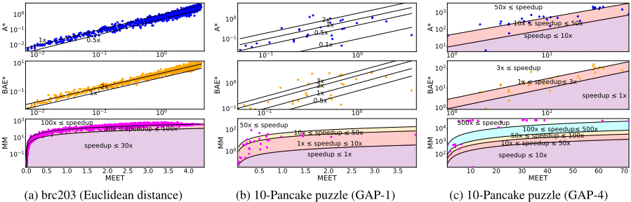
The experimental results demonstrate that MEET significantly improves the search speed as an optimal Bi-HS algorithm, outperforming MM by at least two orders of magnitude (Fig. 4a and Table 1). The runtime of MEET is still on par with A* in brc203d and roughly twice as slow in orz100d. MEET expands slightly more states than BAE* in orz100d but achieves better runtime.
Considering the ablation study, running MEET with the static heuristic h results in similar runtimes compared to running it with ˜h, but the solutions found are often sub-optimal, which aligns with the theory, as the termination conditions TC1-TC4 rely on f-values defined by f = g + ˜h. Finally, the results show that the pruning process reduces the runtime of MEET by an average of roughly 2% over all the instances in grid maps. Results omitted for breivity.
5.2 10-Pancake Puzzle
Our second domain is the well-known Pancake puzzle: A state in the 10-Pancake puzzle is represented by a vector of 10 different numbers, where the goal is to sort them in ascending order through a sequence of flips from a given start state. In our experiments, we apply both GAP, as described in [Helmert, 2010] and GAP-X heuristics [Holte et al., 2017]. The GAP-X heuristics are variants of the original GAP heuristic, devised to be less accurate. GAP-X heuristics exclude gaps that include pancakes among the smallest X in size, where the smallest X in our test dataset is 1. As X increases, GAP-X becomes less accurate. We conduct experiments on 30 random instances, with optimal solution costs (C ∗ ) ranging between 7 and 10.
As indicated by the median search time in Table 1, it is at least 100× faster than MM and an order of magnitude faster than A* as the heuristic accuracy decreases, which suggests the improved efficiency of our algorithm in scenarios with weaker heuristics. Compared to BAE*, MEET consistently achieves better performance, where the performance gap expands with weaker heuristics.
Fig 4b and 4c illustrate the advantages of MEET in runtime over A* and MM. We note that the performance of A* is highly dependent on the accuracy of the heuristic, and when compared to Bi-HS algorithms this dependence is exacerbated, since Bi-HS algorithms also exploit information on g-values from both sides, thus reducing the importance of heuristic accuracy. This explains the dominance of MEET over A* with GAP-X for X > 1.
As for the ablation study, the findings in this domain are consistent with those described for the grid maps domain: optimality can only be guaranteed if ˜h is utilized, and pruning reduces the runtime of MEET by an average of roughly 3%.
Lastly, we analyze differences between the TCs using Fig. 2 and 3. Fig. 2 indicates that TC1, TC3 and TC4 are all frequently triggered in different cases, providing meaningful contributions. Fig. 3 shows that TC3 and TC4 save more runtime as the heuristic weakens, whereas TC1 leads when the heuristic is nearly perfect (e.g., GAP-1). Fig. 3 also shows that it is almost always preferable to use TC2, TC3 and TC4 in addition to TC1 in terms of runtime. This is because the computation time required to evaluate them is insignificant, while the potential runtime reduction is significant.
6 Discussion and FutureWork
While significant progress and achievements have been made in Bi-HS, no algorithm thus far has been able to satisfy MMoptimality while providing competitive runtime. Additionally, the challenge of terminating the search early while still ensuring both optimality and MMP was unsolved. This paper closes these gaps by introducing a new bidirectional best-first search algorithm, MEET, that guarantees MM-optimality with significantly improved runtime compared to MM. Key to the efficiency of our approach is a set of new termination conditions that test states when they are generated and not when they are expanded. A predicate that is computationally cheap to test. This is in contrast to MMwhose termination condition can only be evaluated when a meeting state is expanded.
Interestingly two of the termination conditions (TC3 and TC4) make use of the minimal edge cost ε. This is natural in settings such as grid worlds where many, if not all, edges have the same minimal cost. However, in settings where edge costs can take arbitrary values, these termination conditions can prove to be ineffective. However, by inflating ε by some scalar w, we can use these termination conditions to terminate while ensuring a bounded suboptimal solution whose approximation factor is defined by w. Further exploration of the implication of ε in TC3 and TC4 is left for future work.
Acknowledgments
This research was supported in part by the Technion Autonomous Systems Program (TASP) and by the Israeli Ministry of Science and Technology, grant No. 3-17385.
@inproceedings{ijcai2025p999,
  title     = {Bidirectional Search while Ensuring Meet-In-The-Middle via Effective and Efficient-to-Compute Termination Conditions},
  author    = {Wang, Yi and Weiss, Eyal and Mu, Bingxian and Salzman, Oren},
  booktitle = {Proceedings of the Thirty-Fourth International Joint Conference on
               Artificial Intelligence, {IJCAI-25}},
  publisher = {International Joint Conferences on Artificial Intelligence Organization},
  editor    = {James Kwok},
  pages     = {8987--8995},
  year      = {2025},
  month     = {8},
  note      = {Main Track},
  doi       = {10.24963/ijcai.2025/999},
  url       = {https://doi.org/10.24963/ijcai.2025/999},
}
TY - CPAPER TI - Bidirectional Search while Ensuring Meet-In-The-Middle via Effective and Efficient-to-Compute Termination Conditions AU - Wang, Yi AU - Weiss, Eyal AU - Mu, Bingxian AU - Salzman, Oren T2 - Proceedings of the Thirty-Fourth International Joint Conference on Artificial Intelligence, IJCAI-25 PB - International Joint Conferences on Artificial Intelligence Organization PY - 2025 SP - 8987 EP - 8995 DO - 10.24963/ijcai.2025/999 UR - https://doi.org/10.24963/ijcai.2025/999 ER -Copied
Machine-readable versions of this paper, for tools and AI agents:





