
DeepSTE: Deep Spectral Temporal Embeddings for Dynamic Graph Representation Learning
Proceedings of the Thirty-Fifth International Joint Conference on Artificial Intelligence. Main Track. Pages 2671-2679.
https://doi.org/10.24963/ijcai.2026/297
Keywords
- Data Mining: Mining graphs
- Data Mining: Mining spatial and/or temporal data
Abstract
Temporal embeddings play a crucial role in dynamic graph neural networks (DGNNs) by capturing the temporal dynamics of interactions. However, existing Random Fourier Feature (RFF)-based methods in DGNNs directly sample Fourier frequencies from a fixed, data-independent distribution, neglecting the temporal characteristics of dynamic graphs and thereby limiting representational capacity. We propose DeepSTE, a deep spectral temporal embedding framework for dynamic graphs. DeepSTE learns RFF representations via Monte Carlo importance sampling with a tractable proposal distribution (e.g., Gaussian) to approximate the feature map of a shift-invariant or positive-definite kernel whose latent spectral density is analytically intractable. DeepSTE adopts a data-dependent scale parameter, estimated from interaction intervals, to construct the frequency proposal distribution reflecting time–frequency uncertainty. The frequency DNN and the importance-weighting DNN, initialized from the proposal distribution, are jointly optimized to model the importance-sampled spectral representation and learn adaptive temporal features. Experiments demonstrate the effectiveness of DeepSTE on dynamic link prediction and node classification tasks, while also revealing insights such as temporal embedding decay and accelerated convergence.
- [Cho et al., 2014] Kyunghyun Cho, Bart Van Merriënboer, C ¸aglar Gulc ¸ehre, Dzmitry Bahdanau, Fethi Bougares, Holger Schwenk, and Yoshua Bengio. Learning phrase representations using rnn encoder-decoder for statistical machine translation. In Proceedings of the 2014 confer- ence on empirical methods in natural language processing (EMNLP), pages 1724-1734, 2014.
- [Chung et al., 2025] Hsing-Huan Chung, Shravan Chaud- hari, Xing Han, Yoav Wald, Suchi Saria, and Joydeep Ghosh. Between linear and sinusoidal: Rethinking the time encoder in dynamic graph learning. arXiv preprint arXiv:2504.08129, 2025.
- [Cortes et al., 2010] Corinna Cortes, Mehryar Mohri, and Ameet Talwalkar. On the impact of kernel approxima- tion on learning accuracy. In Proceedings of the thir- teenth international conference on artificial intelligence and statistics, pages 113-120. JMLR Workshop and Con- ference Proceedings, 2010.
- [Feng et al., 2025] ZhengZhao Feng, Rui Wang, TianXing Wang, Mingli Song, Sai Wu, and Shuibing He. A compre- hensive survey of dynamic graph neural networks: Mod- els, frameworks, benchmarks, experiments and challenges. IEEE Transactions on Knowledge and Data Engineering, 2025.
- [Hornik et al., 1989] Kurt Hornik, Maxwell Stinchcombe, and Halbert White. Multilayer feedforward networks are universal approximators. Neural networks, 2(5):359-366, 1989.
- [Huang et al., 2023] Shenyang Huang, Farimah Poursafaei, Jacob Danovitch, Matthias Fey, Weihua Hu, Emanuele Rossi, Jure Leskovec, Michael Bronstein, Guillaume Rabusseau, and Reihaneh Rabbany. Temporal graph benchmark for machine learning on temporal graphs. Advances in Neural Information Processing Systems, 36:2056-2073, 2023.
- [Huang et al., 2025] Xuanwen Huang, Wei Chow, Yize Zhu, Yang Wang, Ziwei Chai, Chunping Wang, Lei Chen, and Yang Yang. Enhancing cross-domain link prediction via evolution process modeling. In Proceedings of the ACM on Web Conference 2025, pages 2158-2171, 2025.
- [Jin et al., 2022] Ming Jin, Yuan-Fang Li, and Shirui Pan. Neural temporal walks: Motif-aware representation learn- ing on continuous-time dynamic graphs. Advances in Neural Information Processing Systems, 35:19874-19886, 2022.
- [Joachims, 2006] Thorsten Joachims. Training linear svms in linear time. In Proceedings of the 12th ACM SIGKDD international conference on Knowledge discovery and data mining, pages 217-226, 2006.
- [Kazemi et al., 2020] Seyed Mehran Kazemi, Rishab Goel, Kshitij Jain, Ivan Kobyzev, Akshay Sethi, Peter Forsyth, and Pascal Poupart. Representation learning for dynamic graphs: A survey. Journal of Machine Learning Research, 21(70):1-73, 2020.
- [Kipf and Welling, 2016] Thomas N Kipf and Max Welling. Semi-supervised classification with graph convolutional networks. arXiv preprint arXiv:1609.02907, 2016.
- [Kumar et al., 2019] Srijan Kumar, Xikun Zhang, and Jure Leskovec. Predicting dynamic embedding trajectory in temporal interaction networks. In Proceedings of the 25th ACM SIGKDD international conference on knowl- edge discovery & data mining, pages 1269-1278, 2019.
- [Li et al., 2019] Yanjun Li, Kai Zhang, Jun Wang, and San- jiv Kumar. Learning adaptive random features. In Pro- ceedings of the AAAI conference on artificial intelligence, volume 33, pages 4229-4236, 2019.
- [Lu et al., 2017] Zhou Lu, Hongming Pu, Feicheng Wang, Zhiqiang Hu, and Liwei Wang. The expressive power of neural networks: A view from the width. Advances in neu- ral information processing systems, 30, 2017.
- [Lu et al., 2022] Mingxuan Lu, Zhichao Han, Susie Xi Rao, Zitao Zhang, Yang Zhao, Yinan Shan, Ramesh Raghu- nathan, Ce Zhang, and Jiawei Jiang. Bright-graph neural networks in real-time fraud detection. In Proceedings of the 31st ACM international conference on information & knowledge management, pages 3342-3351, 2022.
- [Pareja et al., 2020] Aldo Pareja, Giacomo Domeniconi, Jie Chen, Tengfei Ma, Toyotaro Suzumura, Hiroki Kaneza- shi, Tim Kaler, Tao Schardl, and Charles Leiserson. Evolvegcn: Evolving graph convolutional networks for dynamic graphs. In Proceedings of the AAAI conference on artificial intelligence, volume 34, pages 5363-5370, 2020.
- [Qian et al., 2024] Hao Qian, Hongting Zhou, Qian Zhao, Hao Chen, Hongxiang Yao, Jingwei Wang, Ziqi Liu, Fei Yu, Zhiqiang Zhang, and Jun Zhou. Mdgnn: Multi- relational dynamic graph neural network for comprehen- sive and dynamic stock investment prediction. In Proceed- ings of the AAAI Conference on Artificial Intelligence, vol- ume 38, pages 14642-14650, 2024.
- [Rahimi and Recht, 2007] Ali Rahimi and Benjamin Recht. Random features for large-scale kernel machines. Ad- vances in neural information processing systems, 20, 2007.
- [Rossi et al., 2020] Emanuele Rossi, Ben Chamberlain, Fab- rizio Frasca, Davide Eynard, Federico Monti, and Michael Bronstein. Temporal graph networks for deep learning on dynamic graphs. arXiv preprint arXiv:2006.10637, 2020.
- [Si et al., 2017] Si Si, Cho-Jui Hsieh, and Inderjit S Dhillon. Memory efficient kernel approximation. Journal of Ma- chine Learning Research, 18(20):1-32, 2017.
- [Trivedi et al., 2019] Rakshit Trivedi, Mehrdad Farajtabar, Prasenjeet Biswal, and Hongyuan Zha. Dyrep: Learn- ing representations over dynamic graphs. In International conference on learning representations, 2019.
- [Vaswani et al., 2017] Ashish Vaswani, Noam Shazeer, Niki Parmar, Jakob Uszkoreit, Llion Jones, Aidan N Gomez, Łukasz Kaiser, and Illia Polosukhin. Attention is all you need. Advances in neural information processing systems, 30, 2017.
- [Veličković et al., 2017] Petar Veličković, Guillem Cucurull, Arantxa Casanova, Adriana Romero, Pietro Lio, and Yoshua Bengio. Graph attention networks. arXiv preprint arXiv:1710.10903, 2017.
- [Wang et al., 2021a] Xuhong Wang, Ding Lyu, Mengjian Li, Yang Xia, Qi Yang, Xinwen Wang, Xinguang Wang, Ping Cui, Yupu Yang, Bowen Sun, et al. Apan: Asyn- chronous propagation attention network for real-time tem- poral graph embedding. In Proceedings of the 2021 inter- national conference on management of data, pages 2628- 2638, 2021.
- [Wang et al., 2021b] Yanbang Wang, Yen-Yu Chang, Yunyu Liu, Jure Leskovec, and Pan Li. Inductive representa- tion learning in temporal networks via causal anonymous walks. In International Conference on Learning Represen- tations (ICLR), 2021.
- [Wu et al., 2024] Yuxia Wu, Yuan Fang, and Lizi Liao. On the feasibility of simple transformer for dynamic graph modeling. In Proceedings of the ACM web conference 2024, pages 870-880, 2024.
- [Xu et al., 2019] Da Xu, Chuanwei Ruan, Evren Korpeoglu, Sushant Kumar, and Kannan Achan. Self-attention with functional time representation learning. Advances in neu- ral information processing systems, 32, 2019.
- [Xu et al., 2020] Da Xu, Chuanwei Ruan, Evren Korpeoglu, Sushant Kumar, and Kannan Achan. Inductive repre- sentation learning on temporal graphs. arXiv preprint arXiv:2002.07962, 2020.
- [Xu et al., 2021] Da Xu, Chuanwei Ruan, Evren Korpeoglu, Sushant Kumar, and Kannan Achan. A temporal kernel approach for deep learning with continuous-time informa- tion. arXiv preprint arXiv:2103.15213, 2021.
- [Ying et al., 2018] Rex Ying, Ruining He, Kaifeng Chen, Pong Eksombatchai, William L Hamilton, and Jure Leskovec. Graph convolutional neural networks for web- scale recommender systems. In Proceedings of the 24th ACM SIGKDD international conference on knowledge discovery & data mining, pages 974-983, 2018.
- [Yu et al., 2023] Le Yu, Leilei Sun, Bowen Du, and Weifeng Lv. Towards better dynamic graph learning: New architec- ture and unified library. Advances in Neural Information Processing Systems, 36:67686-67700, 2023.
- [Yuan et al., 2025] Qi Yuan, Yang Liu, Yateng Tang, Xin- huan Chen, Xuehao Zheng, Qing He, and Xiang Ao. Dy- namic graph learning with static relations for credit risk assessment. In Proceedings of the AAAI conference on ar- tificial intelligence, volume 39, pages 13133-13141, 2025.
- [Zhang et al., 2022] Mengqi Zhang, Shu Wu, Xueli Yu, Qiang Liu, and Liang Wang. Dynamic graph neural net- works for sequential recommendation. IEEE Transactions on Knowledge and Data Engineering, 35(5):4741-4753, 2022.
- [Zhou et al., 2022] Hongkuan Zhou, Da Zheng, Israt Nisa, Vasileios Ioannidis, Xiang Song, and George Karypis. Tgl: a general framework for temporal gnn training on billion-scale graphs. Proceedings of the VLDB Endow- ment, 15(8):1572-1580, 2022.
References were extracted automatically from the PDF and may contain errors.
Full text extracted automatically from the PDF; figures, tables and equations may differ. The PDF is the version of record.
1 Introduction
Dynamic graphs are prevalent in real-life systems such as social networks, recommender systems, biological interactomes, and financial transaction networks, where the topological structure evolves over time [Kazemi et al., 2020; Pareja et al., 2020; Rossi et al., 2020; Wang et al., 2021a; Lu et al., 2022; Zhang et al., 2022; Huang et al., 2023; Qian et al., 2024; Huang et al., 2025; Yuan et al., 2025]. However, representation learning on dynamic graphs poses significant challenges due to continuous temporal dynamics and evolving graph topology, in contrast to the static and time-invariant nature of conventional graphs [Kipf and Welling, 2016; Veliˇckovi´c et al., 2017; Ying et al., 2018; Xu et al., 2020]. Dynamic graph neural networks (DGNNs), such as TGAT [Xu et al., 2020], TGN [Rossi et al., 2020], APAN [Wang et al., 2021a], CAWN [Wang et al., 2021b], and SimpleDyG [Wu et al., 2024], model dynamic graphs by aggregating information from temporal neighbors. A core component of these models is the temporal embedding kernel, which encodes continuous time to capture latent temporal patterns. For example, on e-commerce platforms, purchases typically reflect long-term interests, while views capture short-term preferences. Since older interactions may be less relevant to the current topology, modeling temporal relevance is crucial for accurate recommendation.
∗Corresponding authors.
Kernel methods, such as Support Vector Machines, offer strong theoretical guarantees and effectively approximate complex nonlinear decision boundaries. However, their scalability to large dynamic graphs is hindered by the high computational and memory overhead of nonlinear kernel evaluations [Joachims, 2006; Cortes et al., 2010; Si et al., 2017; Li et al., 2019]. Random Fourier Features (RFFs) approximate shift-invariant kernels by mapping input data into a randomized feature space via Monte Carlo direct sampling from the prior spectral distribution, e.g., Gaussian and Laplacian kernels. This enables scalable learning by replacing costly kernel matrix decomposition with explicit mappings, allowing efficient linear methods to approximate nonlinear models [Rahimi and Recht, 2007]. To address the limitation of positional encoding in self-attention, which captures discrete orderings but fails to model continuous time, [Xu et al., 2019] propose a translation-invariant time kernel based on RFFs that embeds time spans into high-dimensional representations and enables self-attention to capture temporal patterns. TGAT adopts a learnable linear projection to approximate the frequency components of the Fourier basis in RFFs, enabling the model to dynamically learn the spectral distribution [Xu et al., 2020]. These RFF methods have been widely incorporated into DGNNs to model temporal dynamics in continuous-time edges [Wu et al., 2024].
Despite their success, existing RFF-based methods in DGNNs struggle with two fundamental challenges.
- Data-Independent Direct Sampling. Existing RFF-based methods sample Fourier frequencies from a fixed, dataindependent distribution, neglecting the latent, analytically intractable spectral distribution. This limits the expressiveness of the RFF representations and prevents adaptation to real-world dynamic graphs with complex temporal patterns [Li et al., 2019; Xu et al., 2019; Chung et al., 2025].
- Shallow Temporal Embeddings. Merely using a single linear layer to approximate the frequency component in vanilla RFFs is insufficient to capture complex temporal patterns in dynamic graphs. This limited model depth constrains the ability to learn adaptive temporal embeddings that accurately represent continuous-time edge dynamics.
To address the aforementioned challenges, we propose DEEPSTE, a novel DEEP Spectral Temporal Embedding framework for dynamic graph representation learning, which introduces the following two key advances:
- Data-dependent Importance Sampling. To approximate the analytically intractable spectral density distribution in realworld dynamic graphs, DEEPSTE constructs RFFs via Monte Carlo importance sampling with a tractable, data-dependent proposal distribution (e.g., Gaussian), which is estimated from the empirical distribution of interaction time intervals and reflects the time-frequency uncertainty principle.
- Adaptive Temporal Features. DEEPSTE employs multilayer perceptrons (MLPs) to learn adaptive temporal embeddings. Guaranteed by the generalization error bounds we establish, the frequency DNN and importance-weighting DNN are jointly optimized to approximate non-analytic frequency and importance weighting patterns in importancesampled RFFs, enabling DEEPSTE to capture temporal dynamics through the learnable DNN components. Contributions can be summarized as follows:
- We propose DEEPSTE, a novel deep spectral temporal embedding for dynamic graphs, which reformulates RFFs via data-dependent Monte Carlo importance sampling estimated from interaction time intervals and consistent with the time-frequency uncertainty principle.
- We establish generalization error bounds that guarantee the DEEPSTE design, which employs a frequency initialization DNN and an importance-weighting DNN to approximate shift-invariant positive-definite kernels, enabling the learning of adaptive temporal embeddings.
- Extensive experiments on dynamic graphs show that DEEPSTE improves the dynamic link prediction and node classification tasks by 2.32% and 1.32%, respectively, while uncovering insights on DNN depth, temporal embedding decay effect, and faster convergence.
2 Preliminaries
Dynamic Graphs. A dynamic graph over continuous time t ∈ (0, T ], denoted G(t) = (V(t), E(t)), is defined by a timeordered sequence of edge events: X(t)= (x(t1), . . . , x(tn)). Each event x(ti) ∈ X(t) represents an interaction between nodes ui and vi at time ti with edge feature ei ∈ Re , x(ti)= (ui, vi, ei, ti). The set of neighbors of a node u∈V(t) at time t is defined as Nu(t)={v | (u, v) ∈ E(t)}.
RFFs-based Temporal Embedding. The temporal embedding function ϕ(t) in DGNNs maps the continuous-time t ∈ R into a d-dimensional vector space, ϕ : R → Rd [Xu et al., 2019; Xu et al., 2021]. Random Fourier Features (RFFs) explicitly map inputs into a low-dimensional feature space via Monte Carlo direct sampling from the kernel's prior spectral distribution, resulting in the approximation k(t1, t2) ≈ z(t1)′z(t2) [Rahimi and Recht, 2007; Xu et al., 2019]. Based on Bochner's theorem, any continuous, shift-invariant and positive-definite kernel k(t1, t2) = k(t1 - t2) on Rd can be represented as the Fourier transform of a non-negative finite measure. Specifically, if k is integrable, we have k(t1 - t2) = ∫R eiω(t1-t2)p(ω) dω = Eω[ξω(t1)ξω(t2)∗ ] with spectral density p(ω), feature map ξω(t) = eiωt , and ∗ for complex conjugation. For the real part Re(k(t1 - t2)), we have Eω [cos (ω(t1 - t2))] = Eω [cos(ωt1) cos(ωt2) + sin(ωt1) sin(ωt2)] . This motivates mapping time into a finite-dimensional random feature space:
where ωi i.i.d. ∼ p(ω). By Mercer's theorem, periodic, translation-invariant kernels admit a Fourier decomposition k(t1, t2) = ∑∞j=1 cj zj(t1) zj(t2), where cj are Fourier coefficients and {zj} are the corresponding eigenfunctions. This leads to the Mercer random feature map:
where cj are the kernel's Fourier coefficients. Truncating the expansion and combining multiple frequencies yields the final Mercer temporal embedding function as follows:
3 Deep Spectral Temporal Embeddings
In this section, we present DEEPSTE, a framework that integrates data-dependent Monte Carlo importance sampling with adaptive temporal embeddings learned via DNNs.
3.1 Data-dependent Importance Sampling
Temporal Embedding. By Bochner's theorem, a continuous, shift-invariant kernel k(t1, t2) = k(t1 - t2) admits the Fourier representation, k(t1 - t2) = ⟨ϕ(t1), ϕ(t2)⟩ = ∫R eiω(t1-t2) p(ω) q(ω) q(ω) dω, where q(ω) is a proposal distribution and w(ω) = p(ω) q(ω) is the importance weight with spectral density p(ω). By estimating the real part of the above integral, we obtain the Bochner Fourier features:
For the mercer embedding, we reformulate the kernel as an importance-weighted expectation with Fourier coefficients encoded in the spectral density implicitly, k(t1, t2) =
| Proposal Distribution | Variance | |
|---|---|---|
| Gaussian N (0, σ2 ) | 1 √2πσ2 exp (- ω2 2σ2 ) 1 (- |ω| ) | σ2 |
| Laplace(0, b) | 2b exp b | 2b2 |
| Cauchy(0, γ) | 1 πγ(1+ ω2 γ2 ) | - |
Eω∼q(ω)[ p(ω) q(ω) zω(t1) zω(t2)]. Thus, we obtain the Mercer Fourier features with frequency ω and importance weights:
where w′j ∝ cj p(ωj ) q(ωj) denote the importance weight p(ωj) q(ωj) combined with the Fourier coefficient cj . The full Mercer feature map is constructed by concatenating the sampled blocks corresponding to different frequency components:
where ωj i.i.d. ∼ q(ω), each ϕMωj (t) is a spectral embedding associated with the periodic kernel component kωj .
Data-dependent Proposal Distributions q(ω). Specifically, DEEPSTE uses Gaussian, Laplacian, and Cauchy distributions as proposal distributions q(ω), chosen for their analytical tractability and complementary spectral properties, as summarized in Table 1. The scale parameter of the proposal distribution q(ω) controls the spectral bandwidth and influences the range of frequencies sampled. Instead of using a fixed parameter, we adopt an adaptive data-dependent approach and learn it jointly with the model. To approximate the latent spectral properties of dynamic graphs, we estimate the scale parameter from the empirical distribution of interaction time intervals. According to Claim 1 in [Li et al., 2019], the optimal frequency sampling distribution satisfies
where fe(·) is a positive monotonically increasing function that also depends on the kernel bandwidth, σ2T denotes the variance of the time-interval distribution. This form shows that σT directly controls the spectral concentration of q(ω), with larger σT leading to a sharper decay in ω and thus a more low-frequency-concentrated distribution, consistent with the time-frequency uncertainty principle.
Thus, given a set of i.i.d. normalized time intervals ∆˜
T = {∆˜ t1, . . . , ∆˜ tn} between nodes and their temporal neighbors in dynamic graphs, we rescale the empirical temporal dispersion as ˜σT = √Var(∆˜ T ) + h2 /h, where Var(∆ ˜ T) denotes the empirical variance and h = 1 is a small constant introduced to prevent degenerate scaling and ensure numerical stability. Since prior results suggest that the spectral concentration of q(ω) increases (i.e., corresponding to a smaller scale parameter) with the temporal variance σ2T , the scale of the frequency-domain proposal should decrease accordingly. We therefore adapt the scale parameter ηT ∈ {σ, b, γ} according to the inverse relation Std(ω) ∼ 1 σT . In practice, we adopt
where η0 is a base scale controlling the spectral width. Consequently, the resulting proposal distribution q(ω) adapts to empirical temporal statistics, yielding a data-dependent distribution motivated by Fourier uncertainty intuition governing the spectral behavior with respect to temporal dispersion.
3.2 Learning Adaptive Features via DNNs
To handle complex frequency distributions, and highdimensional features in importance-sampled RFFs, we use MLPs to jointly learn frequencies and their importance weights in an adaptive manner. By the Universal Approximation Theorem [Hornik et al., 1989; Lu et al., 2017], there exists an MLP f can approximate the function with an error bounded by supx∈X |f(x)-ϕ(x)| <ϵ′ . We state the following claim, which provides guidelines for constructing DNNbased RFFs with a guaranteed error bound (see Appendix).
Claim 1. Let X ⊂R be compact, and let k : R×R→R be a continuous, shift-invariant, positive-definite kernel, weights wi =p(ωi)/q(ωi)≤W, σ2 p,q :=Eq[w(ω)2ω2 ]. Let f(t) be the DNN feature map. If ϵ′ ≤ ϵ 2C(√W+√d)(√W+1) , then
Proof Sketch. The key is to decompose the DNN kernel approximation error via an intermediate RFF map:
corresponding to the RFF sampling error and the DNN approximation error, respectively, by the triangle inequality. ❶ Based on prior work [Rahimi and Recht, 2007; Xu et al., 2019], and by Hoeffding's inequality, we derive the former, which attains its minimum at N ⋆=σp,q √ 2tmax ϵ exp( dϵ2 16W 2 ). ❷ For the DNN approximation error, exploiting the 1Lipschitz property of trigonometric functions, we obtain ∣∣√ wi d cos(ωit)-gw,i cos(fω,i(t))∣∣ ≤ √ wi d ∣∣fω,i(t)-ωit∣∣+ ∣∣gw,i - √ wi d ∣∣ ≤ √ Wd ϵ′ω + ϵ′w ≤ (√ Wd + 1)ϵ′ , ϵ′ := max{ϵ′ω , ϵ′w }. Applying the Euclidean norm ∥·∥2 and the inequality √a+b+c ≤ √a+ √b+ √c, gives ∥f(t)-ϕ(t)∥ ≤ C1(√W + √d)ϵ′ . As ∥ϕ(t)∥ ≤ √W, ∥f(t)∥ ≤ C2(√W + 1), utilizing the Cauchy-Schwarz inequality, we obtain supt1,t2∈X |f(t1)′ f(t2)-ϕ(t1)′ϕ(t2)|≤supt1,t2∈X ∥f(t1)- ϕ(t1)∥∥f(t2)∥ + ∥ϕ(t1)∥∥f(t2) - ϕ(t2)∥ ≤ C(√W + √d)(√W + 1)ϵ′ ≤ ϵ/2, gives ϵ′ ≤ ϵ 2C(√W+√d)(√W+1) , where C =C1(C2+1) absorbs all normalization and normaggregation constants.
Algorithm 1: Training process of DEEPSTE Input: Dynamic graph G(V(t), E(t)); proposal distribution q(ω); frequency DNN fω and importance-weighting gw. 1 Scale parameter ηT with Eq. (4). 2 for each layer l = 1, . . . ,L do 3 Sample weight parametersW(l) ∼q(ω; η2T I). 4 Initialize layer l in fω and gw with weightsW(l) . 5 end 6 for iterations from 1 to I do 7 for number of steps do 8 Batch time intervals Tb = (∆t1, . . . , ∆tb). 9 Spectral temporal embedding ϕDNN(Tb) using Bochner Eq. (6) or Mercer Eq. (7). 10 Compute DGNN model loss function LG. 11 Update DNNs fω, gw via ∇fω LG, ∇gw LG. 12 end 13 endGuided by the existing analysis, the importance-sampled Bochner RFF ϕBimp (t) in Equation (1) consists of two components: frequencies sampled from the proposal distribution and their corresponding importance weights. Thus, we employ two DNNs: a frequency DNN fω : R → Rd to simulate frequency components ω, and an importance-weighting gw :R2d →Rd to approximate the square root of corresponding importance weights, √w(ω)/d. To incorporate both the proposal distribution and the data-dependent scale parameter, we initialize the DNN weights using samples from q(ω), aiming to better approximate the underlying sample features. The DEEPSTE Bochner temporal embedding is defined as:
where ⊕ denotes vector concatenation.
Correspondingly, for the importance-sampled Mercer RFF ϕMimp (t) with m Fourier components as introduced in Equation (2), the frequency DNN fω:R→Rd/m, where dmodm= 0, is responsible for learning the reciprocal of spectral frequencies, 1ω . The importance-weighting gw :R2d →Rd aims to approximate the square root of the importance weights combined with the Fourier coefficients, √cw(ω). The DEEPSTE Mercer temporal embedding is defined as:
The harmonic components {kπfω(t)}mk=1 correspond to multiples of the learned base frequency, facilitating approximation of the kernel's spectral density. The cosine and sine terms form a 2d-dimensional intermediate representation, which is transformed by gw to yield the final embedding. Algorithm 1 presents the training procedure of DEEPSTE.
4 Experimental Evaluation
4.1 Experimental Settings
Datasets. The five benchmark datasets, including four small-scale and one large-scale, with time spans of up to
| Dataset | # Nodes | # Edges | dV | dE | tmax | ˜σT |
|---|---|---|---|---|---|---|
| UCI | 2K | 60K | 172 | 100 | 1.67×10⁷ | 3.26 |
| Wikipedia | 9K | 157K | 172 | 172 | 2.68×10⁶ | 1.45 |
| MOOC | 7K | 412K | 172 | 4 | 2.57×10⁶ | 1.75 |
| USLegis | 1K | 60K | 172 | 1 | 1.10×101 | 1.01 |
| StackOverflow | 201K | 5M | 172 | 172 | 6.73×10⁷ | 1.19 |
107 are summarized in Table 2 and introduced in Appendix. For transductive tasks, graphs are chronologically split 70%/15%/15% for training/validation/testing. For inductive tasks, 10% of nodes are masked as unseen, consistent with previous work.
Baselines. We compare DEEPSTE against 5 state-of-the-art temporal embedding methods commonly used in DGNNs, including: the TGAT-Timer [Xu et al., 2020], RNN [Cho et al., 2014], Attention [Vaswani et al., 2017], and two advanced spectral temporal embedding: Sampling-Bochner and Sampling-Mercer [Xu et al., 2019; Xu et al., 2020]. All baselines are built upon six representative backbone DGNNs-including attention-based (e.g., TGAT, APAN), memory-augmented (e.g., TGN), and motif-based models (e.g., CAWN)-as well as two efficient DGNN frameworks, DyG [Wu et al., 2024] and TGL [Zhou et al., 2022], with ROC AUC used as the evaluation metric.
Hyparparameters. The base scale parameter η0 in Equation (4) is set to 0.01. The m in the DEEPSTE-Mercer (7) is set to 4 to evenly partition the embedding dimension. The hidden dimension of the DGNNs is set to 128. The learning rate is set to 0.001, and early stopping is applied with a patience of 3 epochs over 3 runs. Detailed configurations are in the appendix. Experiments were conducted on NVIDIA A800 GPUs. The code for DEEPSTE is publicly available at https://github.com/johnnyhuangcs/DeepSTE.
4.2 Main Results
This section summarizes the experimental results for the dynamic link prediction and node classification tasks.
Dynamic Link Prediction. We compare DEEPSTE against baseline temporal embeddings under both transductive and inductive settings on 4 backbone DGNNs. As shown in Table 3, DEEPSTE consistently outperforms all baseline temporal embeddings across all settings and datasets on all 4 backbone DGNNs, achieving the highest ROC AUC scores. For TGAT, DEEPSTE-Mercer achieves the most significant improvement on the USLegis dataset, yielding an 11.24% increase in ROC AUC over the best-performing baseline (TGAT-Timer). The average improvement on TGAT across all datasets is 5.66%. DEEPSTE consistently outperforms the best baselines across three DGNNs (TGN, CAWN, and APAN), with an average increase of 2.32% across all models and datasets, demonstrating its effectiveness in dynamic link prediction. Notably, on TGAT, DEEPSTE-Mercer achieves the highest ROC AUC scores on 7 out of 8 datasets across both transductive and inductive settings, whereas DEEPSTEBochner attains the top score on only one time. However, on TGN, DEEPSTE-Bochner achieves more top scores than DEEPSTE-Mercer. DEEPSTE-Bochner and DEEPSTEMercer achieve the highest ROC AUC scores 13 and 19 times, respectively, across all settings. This suggests that DEEPSTE-Mercer appears to be more effective at capturing temporal dynamics than DEEPSTE-Bochner. For the baseline temporal embedding methods, we observe that the spectraltemporal method Sampling-Mercer achieves the second-best ROC AUC score three times, while TGAT-Timer and RNN each achieve it twice. Spectral temporal methods appear to be more effective than classical temporal embeddings.
| DGNN | Time Encoder | Transductive | Inductive | ||||||
|---|---|---|---|---|---|---|---|---|---|
| UCI | Wikipedia | MOOC | USLegis | UCI | Wikipedia | MOOC | USLegis | ||
| TGAT | TGAT-Timer RNN Attention Sampling-Bochner Sampling-Mercer DEEPSTE-Bochner DEEPSTE-Mercer | 76.71 ± 0.32 75.51 ± 1.51 54.97 ± 1.97 61.81 ± 1.36 73.16 ± 1.96 81.16 ± 1.76 83.02 ± 1.90 | 75.54 ± 0.48 75.04 ± 0.40 73.30 ± 0.13 72.17 ± 0.27 73.54 ± 0.06 80.44 ± 0.53 80.47 ± 0.08 | 60.23 ± 0.46 60.70 ± 0.23 55.60 ± 0.34 59.66 ± 1.84 59.93 ± 1.44 60.61 ± 0.17 61.10 ± 0.04 | 60.16 ± 1.37 48.47 ± 1.80 43.35 ± 0.49 50.83 ± 1.23 55.94 ± 1.34 61.48 ± 0.45 71.40 ± 1.43 | 67.54 ± 0.08 71.15 ± 0.45 51.93 ± 1.19 58.46 ± 1.39 69.03 ± 1.61 77.76 ± 2.77 80.09 ± 0.62 | 75.39 ± 0.65 74.09 ± 0.27 72.11 ± 0.15 71.01 ± 0.41 75.82 ± 0.14 78.82 ± 0.36 78.62 ± 0.23 | 57.40 ± 0.55 60.15 ± 0.80 54.20 ± 0.75 57.40 ± 0.33 58.05 ± 3.00 60.37 ± 0.09 61.20 ± 0.00 | 56.07 ± 1.36 54.84 ± 1.98 43.70 ± 0.21 49.20 ± 1.62 55.77 ± 0.32 55.09 ± 1.28 65.50 ± 0.31 |
| TGN | TGAT-Timer RNN Attention Sampling-Bochner Sampling-Mercer DEEPSTE-Bochner DEEPSTE-Mercer | 87.52 ± 1.41 87.23 ± 0.29 85.74 ± 0.08 86.41 ± 0.16 86.74 ± 0.10 90.89 ± 0.14 89.23 ± 0.12 | 92.50 ± 2.75 95.81 ± 0.03 95.70 ± 0.03 95.56 ± 0.07 95.69 ± 0.03 98.27 ± 0.00 97.84 ± 0.24 | 87.33 ± 0.77 88.67 ± 0.13 87.74 ± 0.30 78.15 ± 1.68 85.08 ± 0.42 91.63 ± 0.53 89.15 ± 1.75 | 80.86 ± 0.08 77.55 ± 0.17 74.58 ± 0.19 78.44 ± 0.33 76.31 ± 0.60 81.23 ± 0.06 81.27 ± 0.36 | 78.81 ± 1.68 83.86 ± 0.08 82.20 ± 0.83 82.72 ± 0.12 83.07 ± 0.27 85.95 ± 2.06 85.18 ± 0.83 | 90.86 ± 1.68 95.31 ± 0.02 95.17 ± 0.01 94.83 ± 0.04 95.04 ± 0.03 95.45 ± 0.26 95.58 ± 0.64 | 84.46 ± 0.76 87.69 ± 0.83 87.03 ± 0.37 76.80 ± 1.83 85.88 ± 0.29 88.43 ± 1.62 87.35 ± 1.49 | 59.71 ± 0.69 55.58 ± 1.40 59.89 ± 0.70 59.98 ± 0.06 60.23 ± 0.73 60.68 ± 1.44 58.82 ± 1.34 |
| CAWN | TGAT-Timer RNN Attention Sampling-Bochner Sampling-Mercer DEEPSTE-Bochner DEEPSTE-Mercer | 86.69 ± 0.00 85.11 ± 0.02 82.75 ± 0.02 85.32 ± 0.29 83.99 ± 0.05 86.45 ± 0.10 87.08 ± 0.04 | 97.12 ± 0.03 97.17 ± 0.01 96.52 ± 0.03 96.94 ± 0.01 96.87 ± 0.05 97.63 ± 0.02 97.57 ± 0.02 | 67.02 ± 0.02 66.37 ± 0.11 60.97 ± 0.08 63.40 ± 0.22 63.43 ± 0.16 67.22 ± 0.03 67.63 ± 0.03 | 69.40 ± 0.12 84.59 ± 0.11 69.07 ± 0.37 74.37 ± 0.60 75.56 ± 0.82 86.02 ± 0.14 86.55 ± 0.23 | 85.56 ± 0.05 85.02 ± 0.04 81.39 ± 0.04 85.42 ± 0.30 83.94 ± 0.12 86.20 ± 0.13 86.38 ± 0.16 | 97.14 ± 0.06 97.18 ± 0.01 96.31 ± 0.00 96.96 ± 0.00 96.90 ± 0.01 97.64 ± 0.01 97.59 ± 0.00 | 66.46 ± 0.15 65.86 ± 0.08 59.07 ± 0.14 63.49 ± 0.24 63.49 ± 0.25 67.87 ± 0.16 68.46 ± 0.02 | 72.36 ± 0.12 87.45 ± 0.07 71.94 ± 0.24 78.15 ± 0.13 78.79 ± 0.34 87.96 ± 0.17 88.22 ± 0.04 |
| APAN | TGAT-Timer RNN Attention Sampling-Bochner Sampling-Mercer DEEPSTE-Bochner DEEPSTE-Mercer | 75.75 ± 0.61 73.12 ± 0.62 71.59 ± 0.47 74.37 ± 1.80 76.35 ± 0.51 76.38 ± 0.98 76.19 ± 0.26 | 84.45 ± 1.49 86.93 ± 2.36 90.69 ± 0.91 85.54 ± 0.31 87.95 ± 1.78 90.69 ± 0.18 91.04 ± 2.65 | 98.98 ± 0.08 98.10 ± 1.14 99.29 ± 0.04 85.58 ± 1.00 98.72 ± 0.21 99.27 ± 0.23 99.35 ± 0.06 | 75.95 ± 0.92 74.75 ± 1.70 72.47 ± 1.07 71.03 ± 1.25 68.52 ± 1.74 79.94 ± 1.14 79.65 ± 1.35 | 84.01 ± 0.29 82.26 ± 0.75 79.25 ± 0.22 82.56 ± 1.35 83.75 ± 0.11 84.30 ± 1.21 85.03 ± 0.15 | 84.09 ± 1.85 87.27 ± 1.48 92.01 ± 2.13 86.50 ± 2.01 90.69 ± 1.88 93.77 ± 0.79 92.09 ± 1.27 | 99.07 ± 0.23 98.10 ± 1.22 99.34 ± 0.03 80.58 ± 1.10 99.40 ± 0.04 99.32 ± 0.03 99.41 ± 0.13 | 74.50 ± 1.69 82.31 ± 0.96 80.10 ± 2.76 71.24 ± 1.76 64.72 ± 1.06 83.82 ± 1.82 82.66 ± 2.85 |
| Time Encoder | Transductive | Inductive | ||
|---|---|---|---|---|
| DyG | TGL-TGN | DyG | TGL-TGN | |
| TGAT-Timer | 84.33 ± 0.21 | 88.52 ± 0.12 | 67.28 ± 0.24 | 67.31 ± 0.11 |
| RNN | 82.46 ± 0.02 | 87.02 ± 0.00 | 64.91 ± 0.17 | 61.99 ± 0.66 |
| Attention | 77.67 ± 0.60 | 88.26 ± 0.01 | 59.14 ±1.20 | 66.57 ± 0.10 |
| Sampling-B. | 82.23 ± 0.61 | 88.84 ± 0.06 | 60.97 ±1.08 | 66.02 ± 0.03 |
| Sampling-M. | 82.80 ± 0.31 | 89.06 ± 0.08 | 63.33 ± 2.04 | 67.27 ± 0.10 |
| DeepSTE-B. | 85.64 ± 0.00 | 89.46 ± 0.93 | 68.41 ± 0.25 | 67.75 ± 0.19 |
| DeepSTE-M. | 85.34 ± 0.16 | 89.65 ± 0.06 | 68.61 ± 0.35 | 68.24 ± 0.11 |
We further evaluate our method on large-scale dynamic graphs using efficient DGNN models (e.g., DyG and TGLTGN) whose training time does not exceed 10,000 seconds (see appendix for details). As shown in Table 4, our proposed DEEPSTE achieves an average accuracy improvement of 1.04% over the strongest baselines, with a maximum improvement of 1.33%, demonstrating its effectiveness on large dynamic graphs and recent efficient DGNNs.
Dynamic Node Classification. Table 5 shows dynamic node classification results on Wikipedia and MOOC, which have node labels. DEEPSTE consistently achieves the best results across various settings and datasets, generally outperforming baseline temporal embedding methods. DEEPSTEMercer yields its largest performance gain on the MOOC dataset when integrated with the TGAT DGNN backbone, showing a 5.34% increase in ROC AUC compared to the best-performing baseline, Sampling-Mercer. On average, it achieves a 1.32% improvement across all datasets. Similar to the results observed in dynamic link prediction, DEEPSTEMercer consistently outperforms DEEPSTE-Bochner across most experimental settings, achieving the highest ROC AUC scores in 6 out of 8 cases, compared to only 2 for DEEPSTEBochner, suggesting potentially better temporal modeling.
| Time Encoder | TGAT | TGN | CAWN | APAN | ||||
|---|---|---|---|---|---|---|---|---|
| Wikipedia | MOOC | Wikipedia | MOOC | Wikipedia | MOOC | Wikipedia | MOOC | |
| TGAT-Timer | 77.19 ± 1.68 | 54.24 ± 0.24 | 87.74 ± 0.64 | 61.58 ± 0.20 | 77.33 ± 0.91 | 63.56 ± 0.07 | 85.02 ± 0.06 | 66.21 ± 0.10 |
| RNN | 75.57 ± 1.86 | 56.30 ± 0.25 | 84.91 ± 2.09 | 59.28 ± 1.47 | 76.05 ± 0.17 | 64.58 ± 0.05 | 82.89 ± 0.29 | 66.52 ± 1.27 |
| Attention | 76.54 ± 1.25 | 54.94 ± 0.26 | 83.25 ± 1.37 | 61.41 ± 1.91 | 76.20 ± 0.19 | 64.76 ± 0.68 | 84.66 ± 0.86 | 67.83 ± 0.49 |
| Sampling-Bochner | 76.63 ± 1.64 | 55.68 ± 0.72 | 87.07 ± 1.20 | 58.95 ± 0.49 | 75.88 ± 0.12 | 63.89 ± 0.02 | 82.60 ± 0.64 | 65.87 ± 0.33 |
| Sampling-Mercer | 75.86 ± 0.59 | 56.43 ± 0.09 | 87.05 ± 0.65 | 57.54 ± 0.80 | 74.92 ± 0.74 | 63.76 ± 0.51 | 82.39 ± 0.33 | 68.28 ± 0.72 |
| DEEPSTE-Bochner | 77.93 ± 1.92 | 60.66 ± 0.52 | 88.07 ± 0.18 | 61.08 ± 0.22 | 77.78 ± 0.88 | 65.22 ± 1.12 | 84.67 ± 0.36 | 68.36 ± 0.38 |
| DEEPSTE-Mercer | 77.51 ± 1.00 | 61.77 ± 0.62 | 88.42 ± 0.45 | 62.09 ± 0.15 | 77.80 ± 0.74 | 66.87 ± 0.53 | 85.63 ± 0.37 | 67.64 ± 0.43 |
4.3 Micro Experiments
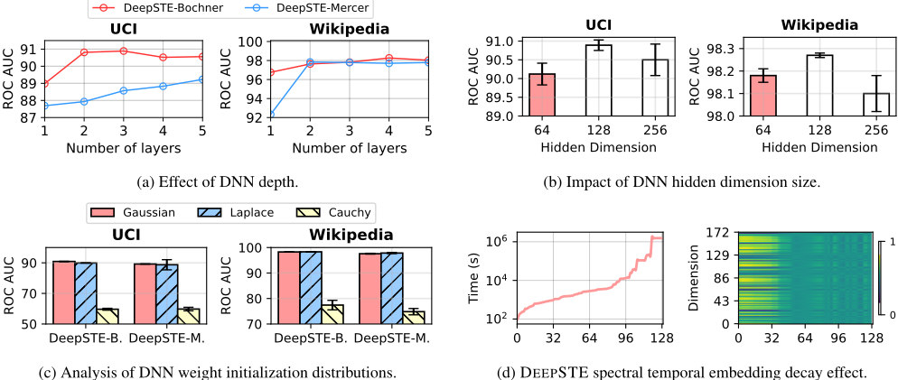
We conduct an in-depth analysis of the impact of various factors on the performance of DGNNs, as shown in Figure 1. Effect of DNN Depth. We investigate the impact of the number of linear layers in the DNNs on the performance of TGN. As shown in Figure 1a, increasing the number of layers generally leads to significantly improved performance compared to using a single linear layer. On the UCI dataset, DEEPSTE-Bochner achieves the best performance with 3 linear layers, while DEEPSTE-Mercer performs best with 5 layers. On the Wikipedia dataset, the corresponding optimal numbers of layers are 4 and 2, respectively. These results show that increasing DNN depth effectively enhances model performance, highlighting the effectiveness of deep models.
Impact of Hidden Dimension Size. Figure 1b illustrates the impact of hidden dimension size in the MLPs on TGN performance. The results show that increasing the hidden dimension generally improves performance, with the optimal result achieved at size 128. This suggests that larger hidden dimensions enhance the DNNs' ability.
Influence of Sampling Distribution. As illustrated in Algorithm 1, the DNN weights are initialized using a proposal distribution q(ω). We analyze the effect of different sampling distributions (Gaussian, Laplace, and Cauchy), with the results presented in Figure 1c. The proposal distribution q(ω) is initialized with a data-driven scale parameter for each dataset, as shown in Table 2. The results indicate that the choice of sampling distribution significantly affects model performance. The Gaussian and Laplace distributions generally yield the best results, while the Cauchy distribution performs the worst. Therefore, the Cauchy distribution may be less suitable as a sampling distribution for Random Fourier Features, as its heavy-tailed characteristics can introduce high variance in the sampled features.
| UCI | Wikipedia | |
|---|---|---|
| DEEPSTE-Bochner | 90.89 ± 0.14 | 98.27 ± 0.00 |
| - (w/o) Data-dependent η - (w/o) Frequency DNN - (w/o) Weight DNN gw - (w) Positional | 87.53 ± 0.76 | 97.72 ± 0.11 |
| fω | 88.87 ± 0.26 | 95.01 ± 0.21 |
| 86.15 ± 0.10 | 96.17 ± 0.07 | |
| embedding | 91.15 ± 0.22 | 98.35 ± 0.15 |
Spectral Temporal Embedding Decay Effect. Figure 1d visualizes the temporal embeddings generated by DEEPSTEBochner on the UCI dataset. The left panel shows 128 interaction intervals, while the right displays the corresponding 172-dimensional temporal embeddings. The model assigns higher weights to recent interactions, with embedding magnitudes decaying and becoming more uniform over time. This indicates a stronger emphasis on temporally close events, potentially enhancing representation learning.
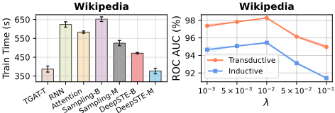
Training Efficiency. Figure 2(a) and the appendix compare DEEPSTE's training efficiency with temporal embedding baselines. DEEPSTE converges in fewer epochs and achieves shorter overall training times. OnWikipedia, DEEPSTE-Mercer achieves the fastest training time and the fewest required epochs. Specifically, DeepSTE-M and DeepSTE-B consistently rank among the top-3 methods in training time across all model-dataset combinations, with mean ranks of 2.83 and 3.25, respectively (see appendix for details).
Scale Parameter Initialization. Figure 2(b) shows the effect of the base scale parameter η0, varied from 10-3 to 10-1 . DEEPSTE performs best at 10-2 , suggesting a favorable balance between high- and low-frequency temporal patterns.
4.4 Ablation Studies
We conduct ablation studies to evaluate the impact of each component in DEEPSTE, as shown in Table 6. Removing the data-driven scale parameter η reduces performance by 3.36% on UCI and 0.55% on Wikipedia, underscoring its importance. Excluding the frequency DNNs fω leads to drops of 2.02% and 3.26%, respectively, indicating the importance of phase information. Eliminating the importanceweighting gw results in declines of 4.74% on UCI and 2.10% on Wikipedia, underscoring the significance of frequencyspecific weighting. Combining DEEPSTE with positional embeddings yields minor gains (0.26% on UCI and 0.08% onWikipedia), suggesting that positional information slightly enhances DGNNs' recognition of ordering information.
5 RelatedWork
DGNNs. DGNNs effectively model dynamic graphs by representing them as event sequences that capture evolving topological structures. Specifically, attention-based DGNNs employ a self-attention mechanism with functional time encoding to capture temporal dependencies and dynamic topological structures [Xu et al., 2020]. TGN represents a continuoustime dynamic graph as a sequence of time-stamped events and leverages a novel combination of memory modules and graph-based operators, using memory-based aggregation and update mechanisms to model temporal dynamics [Rossi et al., 2020]. Motifs-based DGNNs represent temporal networks using causal anonymous walks derived from temporal random walks, capturing temporal motifs in network dynamics [Wang et al., 2021b; Jin et al., 2022]. Recent advanced DGNNs employ Transformer-based architectures with temporal encoding to model temporal dynamics [Wu et al., 2024; Yu et al., 2023; Feng et al., 2025].
Temporal Embedding. The temporal embedding kernel is crucial in DGNNs, enabling the capture of temporal dynamics in contrast to static graphs. Pioneering works employ a single linear layer to project time intervals, thereby enabling the learning of dynamic embedding trajectories or exogenous features in temporal interactions [Kumar et al., 2019; Chung et al., 2025]. Similarly, DyRep also utilizes a linear layer to project time intervals as exogenous features that influence the evolution of embeddings [Trivedi et al., 2019]. RFFbased temporal embeddings use translation-invariant kernels to map continuous time spans into vectors, extending the selfattention mechanism from sequence order to the temporal domain [Xu et al., 2019]. The TGAT timer employs a linear layer to learn the phase patterns of standard RFFs introduced in [Xu et al., 2019], which are subsequently integrated into the attention mechanism [Xu et al., 2020]. This approach has demonstrated strong performance and been widely adopted in later DGNNs for dynamic graph representation learning.
6 Conclusion
We propose DEEPSTE, a deep spectral temporal embedding framework for dynamic graphs that encodes continuous time via Random Fourier Features. The framework employs Monte Carlo importance sampling of the temporal kernel to estimate the target spectral density, together with a data-dependent scale parameter that adapts the frequency distribution of the kernel. Frequency and importanceweighting networks, initialized from proposal distributions, are jointly optimized to learn adaptive temporal embeddings through importance-sampled RFF components. Extensive experiments demonstrated consistent improvements across dynamic link prediction and node classification tasks, while also revealing phenomena such as temporal embedding decay and accelerated convergence for temporal modeling.
Acknowledgments
This work was sponsored by National Natural Science Foundation of China (NO. 62472327, No. 62441229), Key R&D Program of Hubei Province (No. 2023BAB077), and Sichuan Clinical Research Center for Imaging Medicine (YXYX2402).
@inproceedings{ijcai2026p297,
  title     = {DeepSTE: Deep Spectral Temporal Embeddings for Dynamic Graph Representation Learning},
  author    = {Huang, Qiang and Liu, Ke and Gong, Renjie and Zhang, Sijing and Wang, Hao and Feng, Shanshan and Yan, Xiao and Jiang, Jiawei},
  booktitle = {Proceedings of the Thirty-Fifth International Joint Conference on
               Artificial Intelligence, {IJCAI-26}},
  publisher = {International Joint Conferences on Artificial Intelligence Organization},
  editor    = {Diego Calvanese},
  pages     = {2671--2679},
  year      = {2026},
  month     = {8},
  note      = {Main Track},
  doi       = {10.24963/ijcai.2026/297},
  url       = {https://doi.org/10.24963/ijcai.2026/297},
}
TY - CPAPER TI - DeepSTE: Deep Spectral Temporal Embeddings for Dynamic Graph Representation Learning AU - Huang, Qiang AU - Liu, Ke AU - Gong, Renjie AU - Zhang, Sijing AU - Wang, Hao AU - Feng, Shanshan AU - Yan, Xiao AU - Jiang, Jiawei T2 - Proceedings of the Thirty-Fifth International Joint Conference on Artificial Intelligence, IJCAI-26 PB - International Joint Conferences on Artificial Intelligence Organization PY - 2026 SP - 2671 EP - 2679 DO - 10.24963/ijcai.2026/297 UR - https://doi.org/10.24963/ijcai.2026/297 ER -Copied
Machine-readable versions of this paper, for tools and AI agents:





