
MiniST: Unlocking Input Window Length in Traffic Flow Forecasting with Compact Parameters
Proceedings of the Thirty-Fifth International Joint Conference on Artificial Intelligence. Main Track. Pages 2680-2688.
https://doi.org/10.24963/ijcai.2026/298
Keywords
- Data Mining: Mining spatial and/or temporal data
Abstract
Spatiotemporal traffic forecasting currently faces dual challenges: capturing long-range periodic dependencies and managing the computational burden of increasingly complex deep neural network architectures. Mainstream models typically contain millions of parameters and struggle to handle long sequence historical data due to memory bottlenecks. To address these challenges, we present MiniST, a minimalist framework that decouples information content from sequence length by exploiting the intrinsic redundancy of traffic data. Instead of modeling dense point-wise dependencies, MiniST projects high-dimensional traffic history into a compact set of Orthogonal Basis Vectors, effectively distilling dominant traffic modes into a disentangled latent space. Furthermore, we introduce a Template-based Update Module (TUM), which models temporal dynamics by anchoring these latent bases to a set of learnable, time-invariant global templates. Extensive experiments on multiple large-scale datasets, including a network with over 50,000 nodes, demonstrate that MiniST achieves state-of-the-art performance in both short-term and long-term traffic forecasting, outperforming 22 benchmark models with improvements of up to 11.58%, while maintaining minimal parameter size and competitive efficiency.The source code is available at MiniST Repository.
- [Bai et al., 2020] Lei Bai, Lina Yao, Can Li, Xianzhi Wang, and Can Wang. Adaptive graph convolutional recurrent net- work for traffic forecasting. Advances in neural information processing systems, 33:17804-17815, 2020.
- [Benson, 1998] David J Benson. Representations and coho- mology: Volume 1, basic representation theory of finite groups and associative algebras, volume 1. Cambridge university press, 1998.
- [Fang et al., 2023] Yuchen Fang, Yanjun Qin, Haiyong Luo, Fang Zhao, Bingbing Xu, Liang Zeng, and Chenxing Wang. When spatio-temporal meet wavelets: Disentangled traffic forecasting via efficient spectral graph attention networks. In 2023 IEEE 39th international conference on data engi- neering (ICDE), pages 517-529. IEEE, 2023.
- [Fang et al., 2024] Yuchen Fang, Yuxuan Liang, Bo Hui, Zezhi Shao, Liwei Deng, Xu Liu, Xinke Jiang, and Kai Zheng. Efficient large-scale traffic forecasting with trans- formers: A spatial data management perspective. arXiv preprint arXiv:2412.09972, 2024.
- [Han et al., 2024] Jindong Han, Weijia Zhang, Hao Liu, Tao Tao, Naiqiang Tan, and Hui Xiong. Bigst: Linear com- plexity spatio-temporal graph neural network for traffic forecasting on large-scale road networks. Proceedings of the VLDB Endowment, 17(5):1081-1090, 2024.
- [Huang et al., 2023] Qihe Huang, Lei Shen, Ruixin Zhang, Shouhong Ding, Binwu Wang, Zhengyang Zhou, and Yang Wang. Crossgnn: Confronting noisy multivariate time series via cross interaction refinement. Advances in Neural Information Processing Systems, 36:46885-46902, 2023.
- [Huang et al., 2025a] Qihe Huang, Zhengyang Zhou, Kuo Yang, Zhongchao Yi, Xu Wang, and Yang Wang. Timebase: The power of minimalism in efficient long-term time series forecasting. In Forty-second International Conference on Machine Learning, 2025.
- [Huang et al., 2025b] Qihe Huang, Zhengyang Zhou, Kuo Yang, Zhongchao Yi, Xu Wang, and Yang Wang. Timebase: The power of minimalism in long-term time series fore- casting. In Proceedings of the Forty-Second International Conference on Machine Learning (ICML), 2025.
- [Jiang and Luo, 2022] Weiwei Jiang and Jiayun Luo. Graph neural network for traffic forecasting: A survey. Expert systems with applications, 207:117921, 2022.
- [Jin et al., 2023] Guangyin Jin, Yuxuan Liang, Yuchen Fang, Zezhi Shao, Jincai Huang, Junbo Zhang, and Yu Zheng. Spatio-temporal graph neural networks for predictive learn- ing in urban computing: A survey. IEEE transactions on knowledge and data engineering, 36(10):5388-5408, 2023.
- [Kong et al., 2025] Weiyang Kong, Kaiqi Wu, Sen Zhang, and Yubao Liu. Graphsparsenet: a novel method for large scale traffic flow prediction. arXiv preprint arXiv:2502.19823, 2025.
- [Li et al., 2017] Yaguang Li, Rose Yu, Cyrus Shahabi, and Yan Liu. Diffusion convolutional recurrent neural net- work: Data-driven traffic forecasting. arXiv preprint arXiv:1707.01926, 2017.
- [Li et al., 2023] Fuxian Li, Jie Feng, Huan Yan, Guangyin Jin, Fan Yang, Funing Sun, Depeng Jin, and Yong Li. Dynamic graph convolutional recurrent network for traffic prediction: Benchmark and solution. ACM Transactions on Knowledge Discovery from Data, 17(1):1-21, 2023.
- [Lin et al., 2024] Shengsheng Lin, Weiwei Lin, Wentai Wu, Haojun Chen, and Junjie Yang. Sparsetsf: Modeling long- term time series forecasting with 1k parameters. arXiv preprint arXiv:2405.00946, 2024.
- [Liu et al., 2023a] Hangchen Liu, Zheng Dong, Renhe Jiang, Jiewen Deng, Jinliang Deng, Quanjun Chen, and Xuan Song. Staeformer: spatio-temporal adaptive embedding makes vanilla transformer sota for traffic forecasting. arXiv preprint arXiv:2308.10425, 2023.
- [Liu et al., 2023b] Xu Liu, Yutong Xia, Yuxuan Liang, Jun- feng Hu, Yiwei Wang, Lei Bai, Chao Huang, Zhenguang Liu, Bryan Hooi, and Roger Zimmermann. Largest: A benchmark dataset for large-scale traffic forecasting. Advances in Neural Information Processing Systems, 36:75354-75371, 2023.
- [Liu et al., 2023c] Yong Liu, Tengge Hu, Haoran Zhang, Haixu Wu, Shiyu Wang, Lintao Ma, and Mingsheng Long. itransformer: Inverted transformers are effective for time series forecasting. arXiv preprint arXiv:2310.06625, 2023.
- [Ma et al., 2025a] Jiaming Ma, Binwu Wang, Qihe Huang, Guanjun Wang, Pengkun Wang, Zhengyang Zhou, and Yang Wang. Mofo: Empowering long-term time series forecasting with periodic pattern modeling. In The Thirty- ninth Annual Conference on Neural Information Processing Systems, 2025.
- [Ma et al., 2025b] Jiaming Ma, Binwu Wang, Guanjun Wang, Kuo Yang, Zhengyang Zhou, Pengkun Wang, Xu Wang, and Yang Wang. Less but more: Linear adaptive graph learning empowering spatiotemporal forecasting. In The Thirty-ninth Annual Conference on Neural Information Pro- cessing Systems, 2025.
- [Ma et al., 2025c] Jiaming Ma, Binwu Wang, Pengkun Wang, Zhengyang Zhou, Yudong Zhang, Xu Wang, and Yang Wang. Mobimixer: A multi-scale spatiotemporal mixing model for mobile traffic prediction. IEEE Transactions on Mobile Computing, 2025.
- [Nie et al., 2022] Yuqi Nie, Nam H Nguyen, Phanwadee Sinthong, and Jayant Kalagnanam. A time series is worth 64 words: Long-term forecasting with transformers. arXiv preprint arXiv:2211.14730, 2022.
- [Ruan et al., 2025] Weilin Ruan, Xilin Dang, Ziyu Zhou, Sisuo Lyu, and Yuxuan Liang. A retrieval augmented spatio-temporal framework for traffic prediction. arXiv preprint arXiv:2508.16623, 2025.
- [Shao et al., 2022a] Zezhi Shao, Zhao Zhang, Fei Wang, Wei Wei, and Yongjun Xu. Spatial-temporal identity: A simple yet effective baseline for multivariate time series forecast- ing. In Proceedings of the 31st ACM international con- ference on information & knowledge management, pages 4454-4458, 2022.
- [Shao et al., 2022b] Zezhi Shao, Zhao Zhang, Wei Wei, Fei Wang, Yongjun Xu, Xin Cao, and Christian S Jensen. De- coupled dynamic spatial-temporal graph neural network for traffic forecasting. arXiv preprint arXiv:2206.09112, 2022.
- [Shao et al., 2024] Zezhi Shao, Fei Wang, Yongjun Xu, Wei Wei, Chengqing Yu, Zhao Zhang, Di Yao, Tao Sun, Guangyin Jin, Xin Cao, et al. Exploring progress in mul- tivariate time series forecasting: Comprehensive bench- marking and heterogeneity analysis. IEEE Transactions on Knowledge and Data Engineering, 2024.
- [Song et al., 2020] Chao Song, Youfang Lin, Shengnan Guo, and Huaiyu Wan. Spatial-temporal synchronous graph con- volutional networks: A new framework for spatial-temporal network data forecasting. In Proceedings of the AAAI con- ference on artificial intelligence, volume 34, pages 914- 921, 2020.
- [Velikonivtsev et al., 2025] Fedor Velikonivtsev, Oleg Platonov, Gleb Bazhenov, and Liudmila Prokhorenkova. Fine-grained urban traffic forecasting on metropolis-scale road networks. arXiv preprint arXiv:2510.02278, 2025.
- [Wang et al., 2024a] Binwu Wang, Jiaming Ma, Pengkun Wang, Xu Wang, Yudong Zhang, Zhengyang Zhou, and Yang Wang. Stone: A spatio-temporal ood learning frame- work kills both spatial and temporal shifts. In Proceedings of the 30th ACM SIGKDD Conference on Knowledge Dis- covery and Data Mining, pages 2948-2959, 2024.
- [Wang et al., 2024b] Hongjun Wang, Jiyuan Chen, Tong Pan, Zheng Dong, Lingyu Zhang, Renhe Jiang, and Xuan Song. Stgformer: Efficient spatiotemporal graph transformer for traffic forecasting. arXiv preprint arXiv:2410.00385, 2024.
- [Wang et al., 2024c] Shiyu Wang, Haixu Wu, Xiaoming Shi, Tengge Hu, Huakun Luo, Lintao Ma, James Y Zhang, and Jun Zhou. Timemixer: Decomposable mul- tiscale mixing for time series forecasting. arXiv preprint arXiv:2405.14616, 2024.
- [Wu et al., 2019] Zonghan Wu, Shirui Pan, Guodong Long, Jing Jiang, and Chengqi Zhang. Graph wavenet for deep spatial-temporal graph modeling. arXiv preprint arXiv:1906.00121, 2019. IJCAI
- [Wu et al., 2025] Hao Wu, Haomin Wen, Guibin Zhang, Yu- tong Xia, Yuxuan Liang, Yu Zheng, Qingsong Wen, and Kun Wang. Dynst: Dynamic sparse training for resource- constrained spatio-temporal forecasting. In Proceedings of the 31st ACM SIGKDD Conference on Knowledge Discov- ery and Data Mining V. 1, pages 2682-2692, 2025.
- [Xia et al., 2025] Mingyuan Xia, Chunxu Zhang, Zijian Zhang, Hao Miao, Qidong Liu, Yuanshao Zhu, and Bo Yang. Timeemb: A lightweight static-dynamic dis- entanglement framework for time series forecasting. arXiv preprint arXiv:2510.00461, 2025.
- [Xu et al., 2023] Zhijian Xu, Ailing Zeng, and Qiang Xu. Fits: Modeling time series with 10k parameters. arXiv preprint arXiv:2307.03756, 2023.
- [Yao et al., 2019] Huaxiu Yao, Xianfeng Tang, Hua Wei, Guanjie Zheng, and Zhenhui Li. Revisiting spatial-temporal similarity: A deep learning framework for traffic predic- tion. In Proceedings of the AAAI conference on artificial intelligence, volume 33, pages 5668-5675, 2019.
- [Yeh et al., 2024] Chin-Chia Michael Yeh, Yujie Fan, Xin Dai, Uday Singh Saini, Vivian Lai, Prince Osei Aboagye, Junpeng Wang, Huiyuan Chen, Yan Zheng, Zhongfang Zhuang, et al. Rpmixer: Shaking up time series forecasting with random projections for large spatial-temporal data. In Proceedings of the 30th ACM SIGKDD Conference on Knowledge Discovery and Data Mining, pages 3919-3930, 2024.
- [Yu et al., 2017] Bing Yu, Haoteng Yin, and Zhanxing Zhu. Spatio-temporal graph convolutional networks: A deep learning framework for traffic forecasting. arXiv preprint arXiv:1709.04875, 2017. IJCAI
- [Zeng et al., 2023] Ailing Zeng, Muxi Chen, Lei Zhang, and Qiang Xu. Are transformers effective for time series fore- casting? In Proceedings of the AAAI conference on artifi- cial intelligence, volume 37, pages 11121-11128, 2023.
- [Zhang et al., 2023] Xu Zhang, Yongshun Gong, Xinxin Zhang, Xiaoming Wu, Chengqi Zhang, and Xiangjun Dong. Mask-and contrast-enhanced spatio-temporal learning for urban flow prediction. In Proceedings of the 32nd ACM international conference on information and knowledge management, pages 3298-3307, 2023.
- [Zhou et al., 2022] Tian Zhou, Ziqing Ma, Qingsong Wen, Xue Wang, Liang Sun, and Rong Jin. Fedformer: Fre- quency enhanced decomposed transformer for long-term series forecasting. In International conference on machine learning, pages 27268-27286. PMLR, 2022.
References were extracted automatically from the PDF and may contain errors.
Full text extracted automatically from the PDF; figures, tables and equations may differ. The PDF is the version of record.
1 Introduction
Traffic forecasting serves as the cornerstone of Intelligent Transportation Systems (ITS), enabling proactive congestion management and urban resource allocation [Ruan et al., 2025]. The field has witnessed a paradigm shift from classical statistical methods to Spatiotemporal Graph Neural Networks (STGNNs), which have achieved remarkable success by modeling the non-Euclidean correlations among sensors [Jin et al., 2023]. However, this performance gain has come at the cost of escalating architectural complexity [Shao et al., 2024; Wu et al., 2025]. State-of-the-art models typically rely on stacking deep layers with dense pair-wise interaction mechanisms to capture spatiotemporal dependencies. While effective for short horizons, this design creates a "Horizon Bottleneck": the quadratic computational growth prohibits these models from processing long historical input sequences.
∗Binwu Wang and Yang Wang are the corresponding authors.
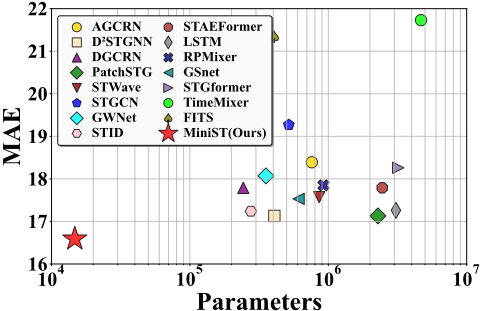
The limitation of the input horizon is a fundamental obstruction to predictive accuracy. Traffic dynamics exhibit intrinsic multi-scale periodicities-ranging from daily commuting rhythms to weekly structural shifts [Yao et al., 2019]. Capturing a complete daily cycle typically requires an input window of hundreds of time steps (e.g., 288 steps for 5-minute intervals) [Shao et al., 2024]. Yet, due to memory and latency constraints, most existing baselines are forced to truncate inputs to short windows (e.g., 12 steps), effectively severing the model's access to global periodic phases. Consequently, while these models may overfit local fluctuations, they struggle to generalize over long-term trends.
High-dimensional traffic data collected frommultiple sensors are in fact governed by only a few sparse, dominant patterns. This perspective is motivated by the strong redundancy present in raw traffic time series: measurements typically exhibit pronounced periodicity, and these patterns remain largely consistent across different sensors. Consequently, modeling each individual data point independently is both computationally expensive and conceptually unnecessary. The key challenge, therefore, is to identify the fundamental components that drive the data and to capture their temporal evolution, thereby addressing current difficulties in a more compact and effective manner.
Guided by this insight, we introduce MiniST, a minimalist spatiotemporal framework that decouples information content from sequence length. MiniST reformulates traffic forecasting as a trajectory evolution process within a compact latent space through two key strategies: ❶ Basis Factorization Strategy: We first distill raw, high-dimensional sequences into a minimal set of Orthogonal Basis Vectors. This step aggressively eliminates redundancy, compressing the input into a Disentangled Feature Space. By enforcing orthogonality, we ensure that these vectors capture mutually independent traffic modes, decoupling the computational cost from the length of the input history. ❷ Template-based Update Module: MiniST employs a template-based update module, where a set of learnable global templates provides a stable reference for capturing recurring macro-periodic patterns while allowing adaptive refinement for local fluctuations. By avoiding deep stacked interaction layers, MiniST achieves favorable accuracy-efficiency trade-offs. Experiments on large-scale benchmarks, including graphs with over 50,000 nodes, demonstrate that MiniST consistently improves forecasting accuracy with significantly fewer parameters and lower runtime. Our contributions are summarized as follows:
- ❶ New Insight. Contrary to the prevailing trend of developing increasingly complex models for performance improvement, this work explores the potential of compact architectures to process long input sequences, thereby empowering traffic flow forecasting.
- ❷ Novel Solution. We propose MiniST, a lightweight architecture that reformulates forecasting as a template-guided reconstruction process. It features a Basis Factorization Strategy to compress redundant inputs into orthogonal components and a Template-based Update Module (TUM) that captures dynamics via global phase anchors and local dictionary atoms.
- ❸ Thorough Experiment. Extensive experiments on realworld datasets demonstrate that MiniST achieves dominant performance in both short-term and long-term traffic flow forecasting tasks.
2 ProblemDefinition
Definition.1 (Traffic Road Network): Traffic road network can be represented as a weighted graph G = (V, E, A), where V is the set of nodes with N nodes. E is the set of edges, and A ∈ RN×N is the adjacency matrix of graph which stores the distances between sensors in the road network G.
Definition.2 (Traffic Flow Tensor): We use Xt ∈ RN to denote the traffic flow of N nodes in the road network observed at timestamp t. We use X = (X1,X2, · · · ,XT ) ∈ RT×N to denote the traffic flow tensor of all nodes over the total T timestamps.
Problem Formalization Given the historical observation data of the past T time steps at time step t, which is denoted as X = (Xt-T+1, · · · ,Xt-1,Xt) ∈ RT×N the goal of the traffic flow forecasting task is to predict the traffic flow in the future T ′ time steps Y = (Xt+1, · · · ,Xt+T ′-1) ∈ RT ′×N .
3 Method
3.1 Overall Framework
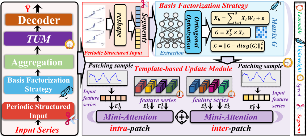
The overall architecture of MiniST is illustrated in Figure 2. MiniST employs two key strategies: the basis decomposition strategy and the basis evolution operator based on canonical memory. MiniST first applies the basis decomposition strategy to decompose the input traffic data X ∈ RT×N into a set of orthogonal basis vectors, retaining key information, represented as Xb ∈ RN×B×lc . This strategy decouples computational complexity from input length. Subsequently, the data is reconstructed into non-overlapping patches, denoted as X ∈ RN×P×L. Following this, the template-based update module is used to efficiently model spatiotemporal dynamics by utilizing a set of canonical memory units, with its output denoted as H ∈ RN×P×L. Finally, H is fed into the decoder to predict future traffic flow.
3.2 Basis Factorization Strategy
Traffic data is characterized by repetitive periodic patterns with high similarity. Our goal is to extract key information from these periodic trends to reduce input complexity. Specifically, we first determine the period length lc. Typically, the period length for traffic data is one day. For instance, with a sampling interval of 5 minutes, lc is equal to 288. Alternatively, the period length lc can be identified using the Fast Fourier Transform. By converting the time series into the frequency domain and examining prominent peaks in the spectrum, periodicity can be determined. For a single sine wave, the period is the reciprocal of its frequency; for a combination of multiple sine waves, the period corresponds to the least common multiple of their individual periods.
Periodic Structured Input. Based on the determined periodic length lc, we structure the input time series of each node Xi ∈ RT into periodic segments Xip ∈ Rm×lc , where i ∈ {1, 2, · · · ,N} and m= ⌈ T lc ⌉ indicates the number of cycles. Notably, if necessary, we use the values from the last time step to fill X to a length of m× lc. Finally, the output of the periodic structure is defined as Xp ∈ RN×m×lc .
Theoretical Motivation: Singular Value Decomposition and Low-Rank Approximation
Given the matrix Xp ∈ Rm×lc , we analyze its inherent lowrank structure through Singular Value Decomposition (SVD). The SVD of Xp is written as
where: U = [u1, . . . , um] ∈ Rm×m is an orthogonal matrix of left singular vectors; V = [v1, . . . , vlc ] ∈ Rlc×lc is an orthogonal matrix of right singular vectors; Σ = diag(σ1, . . . , σr) ∈ Rm×lc contains the singular values; singular values follow
r = rank(Xp) is the matrix rank.
The SVD decomposes Xp into r rank-one components:
Best Low-Rank Approximation. Let
The best rank-B approximation of Xp is
According to the Eckart-Young-Mirsky theorem,
The approximation error is
Learnable Orthogonal Basis. In fact, due to the large number of similar time patterns between each period, the vector Xp is naturally low-rank and contains significant information redundancy. Using such data directly for forecasting models would lead to substantial computational resources being wasted on processing repeated information. However, inspired by the concept of basis representation in linear algebra [Benson, 1998], we can decompose any vector into a linear combination of basis components. This allows us to extract a set of core temporal patterns, known as basis components, from Xp. These basis components can be combined in various ways to reconstruct the original time series data. Specifically, we use linear decomposition method to approximate the basis components,
where W b ∈ Rm×B and W n ∈ Rl×m are learnable weights, and the hyperparameter B is the number of basis components. We then merge the last two dimensions of Xb, and the result is expressed as Xb ∈ RN×Ts , where Ts=B × lc.
Orthogonal Optimization. In data space, the orthogonal relationship between basis vectors enhances their expressive efficiency, allowing any vector to be represented as a linear combination of these vectors. Thus, we apply orthogonality constraints followed by the existing work[Huang et al., 2025b]. These constraints encourage the model to learn varied and distinct time basis components, preventing the absorption of overly singular time series patterns. Specifically, this target loss can be expressed as follows,
where G represents the gram matrix of Xb, and ∥ · ∥2F denotes the Frobenius norm.
3.3 Template-based Update Module
Although we decompose the input into latent basis components XB, these components only represent snapshot states of the traffic network at specific instances. To model how these states evolve over time, we require a stable reference that captures the general regularities of traffic dynamics. Therefore, the core innovation of the Template-based Update Module (TUM) lies in constructing a canonical memory bank of patterns. Instead of computing volatile point-wise dependencies, TUM anchors the drifting basis components to a set of learnable, time-invariant pattern templates.
Patch Segmentation
The patching strategy segments the sequence into small-scale, consecutive patches, thereby preserving contextual temporal information while significantly reducing the computational complexity of downstream temporal modeling [Nie et al., 2022; Wang et al., 2024c]. Specifically, we initially utilize a 1D convolution to aggregate contextual information from Xb ∈ RN×Ts , employing zero-padding to ensure alignment of sequence lengths, and the output is denoted as ˜Xb. Finally, we generate the patch-structured sequence by downsampling after summing the two vectors Xb and ˜Xb, and the output is denoted as X ∈ RN×P×L, where L represents the length of each patch and P = ⌈ Ts L ⌉ represents the number of patches.
Template-based Update Module
❶ Inter-patch Phase Alignment. Traffic dynamics typically follow periodic patterns whose phases drift relative to absolute time. To ground these drifting states, we introduce a set of Global Phase Anchors, parameterized as learnable, time-invariant matrices Dt ∈ RP×L and Ds ∈ RP×L. These anchors act as a canonical reference frame, encoding the stationary evolution modes of urban rhythms. The alignment process projects the drifting input bases onto this stable reference to compute a phase correction term:
Here, the ReLU activation is deliberately employed to enforce sparsity, effectively filtering out weak or noisy interactions between the input state and the global anchors.
❷ Intra-patch Dynamic Refinement. Complementary to the global phase alignment, we establish a Local Invariant Dictionary to capture micro-scale shape fluctuations (e.g., sudden congestion waves). We define Bp ∈ RK×L and Br ∈ RK×L as learnable Dictionary Atoms, which serve as fundamental shape primitives. Instead of modeling these volatile fluctuations directly, we reconstruct them by matching the local input windows against these static atoms. The refinement process is formulated as:
This mechanism allows the model to "lookup" and synthesize complex local dynamics from a compact set of basic primitives, further stabilizing the prediction against random noise.
❸ Dual-Pathway Integration. we add the two representations together to get the final output, which is denoted as H. The complete formula is as follows,
The final representation H represents the traffic state after being calibrated against both the global phase anchors and the local dictionary atoms. By relying on these parameterized invariant references rather than data-dependent attention maps, the BEO achieves a profound reduction in complexity.
Finally, the refined representation H ∈ RN×P×L is fed into the decoder to generate the final predictions. We adopt an MLP-based decoder and use the mean squared error (MSE) to measure the discrepancy between the predictions and the ground truth, denoted as Lp. In summary, our overall optimization objective is formulated as:
where λ is a balance hyperparameter.
| Dataset | # Nodes | # Edges | Time period | Data points |
|---|---|---|---|---|
| PeMS04 | 307 | 338 | 01/01/2018 ∼ 02/28/2018 | 5.22M |
| PeMS08 | 170 | 276 | 07/01/2016 ∼ 08/31/2016 | 3.04M |
| METR-LA | 207 | 1,515 | 03/01/2012 ∼ 06/27/2012 | 7.09M |
| SD | 716 | 17,319 | 01/01/2017 ∼ 12/31/2021 | 0.38B |
| GBA | 2,352 | 61,246 | 01/01/2017 ∼ 12/31/2021 | 1.24B |
| GLA | 3,834 | 98,703 | 01/01/2017 ∼ 12/31/2021 | 2.02B |
| CA | 8,600 | 201,363 | 01/01/2017 ∼ 12/31/2021 | 4.52B |
| City-Traffic-M | 53,530 | 121,236 | 07/01/2024 ∼ 11/01/2024 | 1.78B |
4 Experiment
4.1 Experiment Setup
Dataset We conduct experiments on the following datasets: LargeST [Liu et al., 2023b], METR-LA [Li et al., 2017], PEMS04, PEMS08 [Song et al., 2020], and City-Traffic-M dataset [Velikonivtsev et al., 2025]. Specifically, METRLA consists of 207 traffic sensors; the PEMS dataset covers PEMS04 with 307 sensors and PEMS08 with 170 sensors. City-Traffic-M dataset [Velikonivtsev et al., 2025] is currently the largest traffic dataset, containing 53,530 nodes and 121,236 edges. Detailed statistics are shown in Table 1.
Baseline The experiment included the following advanced traffic prediction baselines: ❶ Time series forecasting models include LSTM, iTransformer [Liu et al., 2023c], Sparsesf [Lin et al., 2024], TimeMixer [Wang et al., 2024c], DLinear [Zeng et al., 2023], NLinear [Zeng et al., 2023], CrossGNN [Huang et al., 2023], PatchTST [Nie et al., 2022], FITS[Xu et al., 2023], RPMixer [Yeh et al., 2024], TimeEmb [Xia et al., 2025], and TimeBase [Huang et al., 2025a]. ❷ Spatiotemporal graph convolutional models include AGCRN [Bai et al., 2020], D2STGNN [Shao et al., 2022b], DGCRN [Li et al., 2023], PatchSTG [Fang et al., 2024], STWave [Fang et al., 2023], STGCN [Yu et al., 2017], GWNet [Wu et al., 2019], STGformer [Wang et al., 2024b], GSnet [Kong et al., 2025], BigST [Han et al., 2024], STAEFormer [Liu et al., 2023a], and STID [Shao et al., 2022a].
Setting All datasets are divided into training, validation, and test sets in a 6:2:2 ratio. We implement all models using the PyTorch framework in Python 3.10 and train them on an NVIDIA A100-80GB GPU with the Adam optimizer. The learning rate for the experiments was set to 0.0025, with a maximum of 200 epochs and an early stopping mechanism in place. Our experiments are based on the LargeST framework [Liu et al., 2023b], where the cycle length is set to lc = 96, and the total number of regularization basis vectors B is set to 6. The length of each patch L is set to 12, and K is set to 16. λ is set to 0.04. We use Mean Absolute Error (MAE), Root Mean Square Error (RMSE), and Mean Absolute Percentage Error (MAPE) as evaluation metrics.
Fairness Statement We set the forecasting horizon to 96 for long-term forecasting and to 12 for short-term forecasting. In order to ensure fair comparisons, we adjust the input length for all baseline models. Specifically, for each model, we fix all other parameters, then determine the optimal input length within the GPU memory constraints and report the corresponding forecasting performance.
| Model | SD | GBA | GLA | PEMS04 | METR-LA | ||||||||||||||||
|---|---|---|---|---|---|---|---|---|---|---|---|---|---|---|---|---|---|---|---|---|---|
| MAE | RMSE | MAPE | MAE | RMSE | MAPE | MAE | RMSE | MAPE | MAE | CA RMSE | MAPE | MAE | RMSE | MAPE | MAE | PEMS08 RMSE MAPE | MAE | RMSE | MAPE | ||
| AGCRN | 18.39 | 33.63 | 13.78 | 20.69 | 34.30 | 16.05 | 20.26 | 64.86 | 12.39 | - | - | - | 17.15 | 27.89 | 13.61 | 14.18 | 24.58 | 8.92 | 3.69 | 8.04 | 11.62 |
| D2STGNN | 17.11 | 28.60 | 12.15 | 21.31 | 34.09 | 16.08 | - | - | - | - | - | - | 18.02 | 28.74 | 15.02 | 14.51 | 23.94 | 9.47 | 3.71 | 7.91 | 11.19 |
| DGCRN | 17.79 | 29.31 | 12.33 | 20.53 | 33.40 | 16.79 | - | - | - | - | - | - | 17.51 | 27.72 | 13.71 | 14.62 | 24.07 | 10.06 | 3.71 | 8.21 | 11.78 |
| PatchSTG | 17.13 | 28.75 | 11.03 | 19.75 | 33.17 | 14.98 | 19.30 | 32.28 | 11.38 | 17.68 | 29.72 | 12.86 | 17.32 | 27.31 | 14.02 | 15.22 | 23.78 | 9.66 | 4.08 | 8.46 | 12.77 |
| STWave | 17.57 | 28.99 | 11.94 | 20.56 | 33.58 | 15.14 | 20.22 | 33.03 | 12.38 | 20.67 | 33.12 | 15.76 | 16.96 | 27.41 | 13.71 | 13.66 | 23.61 | 9.03 | 3.98 | 8.04 | 11.66 |
| STGCN | 19.27 | 33.57 | 13.49 | 23.29 | 38.15 | 17.82 | 22.22 | 37.98 | 14.30 | 20.68 | 35.68 | 15.55 | 16.94 | 27.63 | 13.61 | 14.82 | 24.80 | 9.69 | 3.54 | 7.94 | 11.38 |
| GWNet | 18.07 | 29.97 | 12.70 | 20.83 | 33.37 | 17.30 | 20.37 | 32.65 | 12.71 | 19.75 | 31.71 | 15.84 | 17.84 | 28.26 | 14.87 | 13.91 | 23.21 | 11.97 | 3.59 | 7.91 | 11.18 |
| BigST | 17.17 | 28.63 | 11.94 | 19.09 | 31.41 | 15.57 | 19.50 | 32.07 | 12.91 | 18.23 | 30.43 | 13.91 | 16.88 | 27.13 | 13.38 | 14.06 | 23.76 | 9.31 | 3.65 | 7.85 | 11.83 |
| STAEFormer | 17.79 | 29.69 | 11.65 | 21.30 | 34.56 | 17.63 | - | - | - | - | - | - | 17.75 | 28.15 | 13.94 | 15.22 | 24.81 | 9.41 | 3.61 | 7.89 | 11.32 |
| GSnet | 17.53 | 29.65 | 12.52 | 18.96 | 31.21 | 15.93 | 18.62 | 30.82 | 12.39 | 17.30 | 28.56 | 13.65 | 16.94 | 27.15 | 13.91 | 13.25 | 22.88 | 9.05 | 3.81 | 7.84 | 12.28 |
| STID | 17.24 | 29.39 | 12.31 | 18.50 | 31.20 | 15.34 | 18.15 | 30.01 | 11.87 | 17.06 | 28.97 | 13.32 | 16.89 | 27.22 | 12.76 | 13.08 | 22.92 | 8.93 | 3.63 | 8.09 | 11.88 |
| STGformer | 18.26 | 30.77 | 12.35 | 20.51 | 33.74 | 15.89 | 19.68 | 32.24 | 12.86 | 19.92 | 32.97 | 15.92 | 17.02 | 27.36 | 13.35 | 13.62 | 22.82 | 8.96 | 3.60 | 7.97 | 11.62 |
| LSTM | 17.26 | 28.67 | 11.26 | 19.03 | 32.20 | 14.33 | 18.81 | 31.18 | 11.33 | 23.02 | 36.92 | 18.19 | 18.35 | 29.51 | 14.76 | 13.35 | 22.85 | 9.43 | 4.38 | 9.16 | 14.68 |
| Sparsestf | 25.90 | 46.77 | 18.30 | 26.01 | 45.28 | 21.82 | 25.14 | 44.59 | 17.32 | 23.75 | 43.03 | 18.87 | 22.24 | 38.65 | 17.25 | 16.61 | 30.84 | 11.54 | 8.78 | 13.32 | 21.55 |
| RPMixer | 17.70 | 28.66 | 12.33 | 19.46 | 31.24 | 16.13 | 19.13 | 30.46 | 12.73 | 18.22 | 29.48 | 14.33 | 19.71 | 30.30 | 18.87 | 17.48 | 27.41 | 12.65 | 4.80 | 9.74 | 15.44 |
| TimeMixer | 21.73 | 38.01 | 15.67 | 23.98 | 36.49 | 25.12 | 24.94 | 38.07 | 20.09 | 26.01 | 38.41 | 33.67 | 21.45 | 33.63 | 21.97 | 17.71 | 27.74 | 15.29 | 4.40 | 8.91 | 14.45 |
| PatchTST | 32.91 | 49.79 | 29.56 | 31.77 | 48.33 | 28.87 | 32.63 | 49.88 | 25.24 | 33.65 | 60.43 | 25.92 | 33.66 | 52.11 | 27.84 | 31.36 | 47.01 | 6.93 | 12.68 | 22.89 | |
| iTransformer | 42.23 | 53.80 | 31.10 | 66.63 | 89.46 | 82.62 | 47.65 | 72.97 | 47.45 | - | - | - | 41.04 | 59.93 | 38.85 | 37.81 | 57.62 | 21.83 23.43 | 9.14 | 15.54 | 28.54 |
| FITS | 21.34 | 38.01 | 14.36 | 22.37 | 37.67 | 19.05 | 21.66 | 37.42 | 14.81 | 20.12 | 35.22 | 15.81 | 20.02 | 33.31 | 16.49 | 15.43 | 26.34 | 10.75 | 7.55 | 10.84 | 19.54 |
| DLinear | 21.11 | 37.94 | 14.42 | 22.33 | 37.60 | 18.69 | 21.61 | 37.12 | 16.01 | 20.24 | 35.20 | 17.02 | 25.52 | 41.73 | 19.64 | 22.60 | 37.34 | 14.86 | 6.50 | 11.26 | 18.71 |
| NLinear | 21.15 | 37.98 | 14.33 | 22.22 | 37.31 | 18.82 | 21.54 | 37.03 | 14.67 | 20.23 | 35.40 | 16.01 | 25.60 | 42.03 | 19.68 | 22.66 | 37.54 | 14.89 | 6.97 | 12.42 | 17.80 |
| CrossGNN | 23.09 | 39.04 | 15.87 | 27.01 | 43.31 | 22.38 | 26.79 | 41.55 | 21.12 | 26.16 | 41.25 | 20.25 | 25.11 | 40.32 | 20.88 | 21.91 | 16.73 | 4.98 | 9.82 | 16.51 | |
| TimeBase | 19.15 | 32.21 | 13.22 | 21.11 | 34.51 | 17.12 | 20.67 | 32.55 | 15.76 | 20.23 | 32.43 | 14.42 | 23.21 | 41.59 | 16.18 | 17.52 | 35.69 35.99 | 11.98 | 8.83 | 12.31 | 21.96 |
| TimeEmb | 18.82 | 30.71 | 20.59 | 33.51 | 16.54 | 19.62 | 31.22 | 12.77 | 31.41 | 12.78 | 29.37 | 13.12 | 22.76 | 9.79 | 4.91 | 8.58 | 13.98 | ||||
| 12.55 | 19.12 | 17.17 | 13.96 | ||||||||||||||||||
| Ours | 16.59 | 28.30 | 10.72 | 17.92 | 30.77 | 13.85 | 16.89 | 28.90 | 10.47 | 15.79 | 27.35 | 11.44 | 16.35 | 26.98 | 11.71 | 12.32 | 21.44 | 8.59 | 3.51 | 7.81 | 11.01 |
| Improvement | 3.04% | 1.15% | 2.81% | 5.49% | 0.80% | 7.54% | 6.94% | 3.70% | 7.60% | 7.44% | 4.24% | 11.04% | 3.13% | 0.55% | 8.23% | 5.81% | 6.04% | 3.70% 0.85% | 0.38% | 1.52% | |
| Model | SD | GBA | GLA | PEMS04 | PEMS08 | METR-LA | |||||||||||||||
|---|---|---|---|---|---|---|---|---|---|---|---|---|---|---|---|---|---|---|---|---|---|
| MAE | RMSE | MAPE | MAE | RMSE | MAPE | MAE | RMSE | MAPE | MAE | CA RMSE | MAPE | MAE | RMSE | MAPE | MAE | RMSE | MAPE | MAE | RMSE | MAPE | |
| AGCRN | 26.79 | 50.95 | 20.65 | 28.09 | 47.01 | 25.08 | 28.56 | 49.30 | 19.53 | - | - | - | 21.55 | 34.51 | 17.29 | 17.97 | 31.31 | 11.42 | 4.05 | 8.62 | 13.51 |
| PatchSTG | 23.93 | 46.25 | 16.92 | 25.94 | 44.79 | 22.84 | 25.18 | 44.70 | 18.06 | 23.39 | 41.62 | 19.92 | 21.11 | 35.55 | 17.88 | 17.21 | 29.67 | 12.11 | 5.21 | 9.26 | 15.23 |
| STGCN | 28.64 | 51.55 | 20.23 | 28.63 | 51.55 | 20.23 | 31.09 | 54.10 | 21.36 | 28.36 | 49.53 | 23.30 | 21.39 | 36.08 | 16.53 | 18.27 | 31.44 | 11.53 | 4.01 | 8.68 | 13.62 |
| GWNet | 27.33 | 47.99 | 20.43 | 27.33 | 47.98 | 20.43 | 34.09 | 52.69 | 22.08 | 28.72 | 47.12 | 25.28 | 20.90 | 35.51 | 17.21 | 17.80 | 30.31 | 13.24 | 3.99 | 8.62 | 13.55 |
| BigST | 23.78 | 41.91 | 18.45 | 25.08 | 41.59 | 24.19 | 25.56 | 43.09 | 19.16 | 23.51 | 39.83 | 21.01 | 23.11 | 37.83 | 19.34 | 19.23 | 32.57 | 12.78 | 4.80 | 8.62 | 13.92 |
| STID | 23.20 | 42.49 | 17.38 | 23.82 | 47.93 | 27.21 | 23.43 | 41.45 | 16.92 | 22.23 | 39.14 | 18.73 | 21.31 | 35.29 | 16.86 | 15.83 | 27.69 | 11.72 | 3.87 | 8.44 | 13.38 |
| GSnet | 23.74 | 42.27 | 17.29 | 25.85 | 42.03 | 23.44 | 24.65 | 40.98 | 18.01 | 23.08 | 38.26 | 19.30 | 21.13 | 33.89 | 17.77 | 17.37 | 29.35 | 12.70 | 4.23 | 8.72 | 14.35 |
| STGformer | 26.79 | 48.49 | 18.54 | 29.72 | 48.04 | 26.12 | 29.92 | 49.69 | 21.01 | 28.02 | 47.32 | 22.86 | 21.05 | 34.16 | 16.59 | 17.36 | 29.84 | 11.58 | 3.96 | 8.57 | 13.71 |
| LSTM | 24.66 | 42.46 | 16.51 | 29.12 | 42.07 | 20.03 | 29.12 | 47.93 | 27.21 | 35.12 | 55.48 | 29.30 | 22.26 | 36.71 | 17.97 | 17.63 | 30.67 | 12.90 | 4.75 | 9.83 | 16.25 |
| Sparsestf | 26.46 | 50.27 | 17.14 | 27.44 | 48.22 | 23.16 | 27.06 | 48.72 | 19.18 | 25.59 | 45.56 | 21.11 | 23.86 | 40.34 | 20.77 | 18.08 | 34.63 | 13.21 | 9.66 | 15.72 | 21.97 |
| RPMixer | 24.70 | 41.05 | 18.24 | 25.85 | 42.94 | 22.79 | 25.97 | 42.86 | 18.33 | 24.01 | 40.06 | 20.84 | 21.60 | 35.93 | 17.85 | 18.12 | 31.78 | 13.11 | 5.45 | 10.52 | 18.44 |
| TimeMixer | 31.61 | 49.91 | 29.68 | 33.11 | 53.51 | 30.94 | 35.95 | 55.08 | 39.15 | 35.86 | 59.77 | 29.36 | 31.46 | 50.58 | 35.01 | 24.93 | 39.80 | 30.57 | 5.02 | 9.93 | 16.69 |
| PatchTST | 60.12 | 89.12 | 57.16 | 52.07 | 79.36 | 59.33 | 53.28 | 82.33 | 48.31 | 60.11 | 80.44 | 55.16 | 36.02 | 57.93 | 31.76 | 47.57 | 62.85 | 28.63 | 7.72 | 13.97 | 25.72 |
| iTransformer | 55.25 | 83.72 | 40.54 | 50.20 | 73.63 | 50.06 | 53.19 | 77.40 | 48.85 | - | - | - | 47.09 | 70.67 | 45.67 | 42.60 | 63.73 | 29.70 | 9.34 | 15.95 | 28.47 |
| FITS | 25.70 | 48.99 | 16.76 | 26.17 | 46.64 | 21.19 | 25.54 | 46.85 | 17.17 | 23.91 | 44.27 | 18.40 | 22.54 | 40.49 | 17.08 | 16.85 | 33.80 | 11.76 | 8.38 | 11.70 | 21.04 |
| DLinear | 26.15 | 49.11 | 18.06 | 27.72 | 47.43 | 24.30 | 27.20 | 47.51 | 21.16 | 25.23 | 44.79 | 21.53 | 32.96 | 56.39 | 25.62 | 30.97 | 53.47 | 21.67 | 7.76 | 12.69 | 23.89 |
| NLinear | 26.01 | 48.98 | 17.51 | 27.71 | 47.43 | 24.46 | 26.86 | 47.45 | 19.06 | 25.24 | 44.79 | 20.93 | 33.02 | 56.47 | 25.43 | 30.94 | 53.55 | 8.87 | 16.01 | 21.80 | |
| CrossGNN | 30.49 | 50.97 | 21.01 | 39.58 | 62.43 | 34.71 | 42.21 | 65.41 | 30.64 | 38.29 | 60.75 | 32.98 | 36.36 | 58.18 | 31.13 | 33.51 | 53.53 | 20.71 | 6.79 | 12.39 | 23.5 |
| TimeBase | 24.89 | 42.77 | 17.56 | 26.92 | 45.14 | 21.07 | 26.29 | 44.34 | 17.68 | 25.54 | 44.12 | 18.26 | 23.31 | 41.77 | 16.73 | 17.71 | 35.83 | 24.65 12.21 | 9.09 | 12.44 | 22.54 |
| TimeEmb | 24.56 | 42.65 | 25.92 | 44.02 | 24.76 | 17.23 | 24.11 | 42.78 | 18.85 | 20.92 | 35.69 | 15.84 | 27.85 | 12.15 | 5.18 | ||||||
| 17.34 | 21.69 | 43.43 | 16.64 | 9.02 | 15.31 | ||||||||||||||||
| Ours | 21.94 | 40.78 | 15.50 | 21.84 | 38.46 | 18.77 | 21.72 | 39.46 | 14.96 | 20.87 | 37.62 | 17.04 | 20.84 | 34.08 | 16.29 | 15.64 | 27.37 | 11.41 | 3.91 | 8.37 | 13.21 |
| improvement | 5.43% | 0.66% | 8.39% | 8.31% | 7.52% | 6.29% | 7.30% | 3.70% | 11.58% | 6.12% | 1.67% | 9.02% | 0.29% | 0.23% | 1.45% | 1.20% | 1.16% | 1.58% | 2.01% | 0.83% | 1.27% |
4.2 Experiment Result Analysis
Short-termPerformance Comparison In Table 2, we report the average performance over 12 time steps in short-term forecasting tasks. Time series forecasting models typically underperform compared to STGNNs due to their inability to explicitly capture spatial dependencies. Among time series models, RPMixer leverages the ensemble learning capabilities of deep neural networks to effectively model complex temporal dependencies, achieving relatively good performance in the time series domain. However, in the realm of STGNN models, complex architectures like D2STGNN and STAEFormer face scalability issues in small traffic networks and perform poorly on large datasets, occasionally failing to function altogether. In contrast, BigST and GSNet utilize efficient graph structure learning techniques to reduce computational complexity. Notably, some spatiotemporal models based on MLPs, such as STID-which combines MLP with spatiotemporal embedding techniques-demonstrate impressive performance and excellent scalability.
Long-term Performance Comparison In Table 3, we report the average long-term forecasting performance over 96 forecasting time steps. Some time series models expected to excel in long-term forecasting, such as TimeMixer and iTransformer, do not perform as well as most STGNNs, highlighting the importance of spatial modeling for traffic forecasting tasks. SparseSTF enhances its long-term forecast performance by using downsampling techniques on the original sequences, effectively capturing periodic patterns, and thus outperforms its short-term forecast capabilities. Models with high parameter complexity, particularly those based on Transformers like STAEFormer and D2STGNN, struggle with long-term forecasting tasks. In contrast, GSNet and BigST deliver excellent performance due to their lightweight graph learning designs that accurately model spatiotemporal dependencies in longer historical sequences.
In summary, our MiniST model achieves competitive predictive performance in both short-term and long-term traffic forecasting tasks. Notably, our model enhances performance by up to 11.58%.
4.3 Ablation Experiment
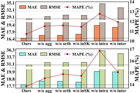
We conduct ablation experiments on both the SD and GBA datasets. There are six variants: (1) "w/o agg" (mean that we remove context information aggregation), (2) "w/o orth" (removing the regularization operation), (3) "w/o inSK" (removing input basis component extraction.), (4) "w/o intra" (removing intra-patch dependency modeling), and (5) "w/o inter" (removing inter-patch dependency modeling), (6)"rl2sm" (replacing the activation function ReLU with Softmax).
As shown in Figure 3, our complete model achieves the best performance across all metrics on both SD and GBA datasets. "w/o agg" results reveal that removing the aggregation module degrades performance, as aggregation enriches contextual information and suppresses outliers, improving stability and accuracy. "w/o inSK" variant also performs worse, confirming that inSK captures essential periodic patterns for stable feature learning, while the orthogonal operation refines the extracted features. Notably, "w/o intra" and w/o inter yield the largest errors, underscoring the critical role of intra-patch and inter-patch dependencies: the former captures local temporal dynamics, while the latter models long-range dependencies across patches. "rl2sm variant" performs poorly because traffic dependencies are inherently non-negative and sparse. Unlike Softmax, which over-amplifies noise through global normalization, ReLU effectively preserves strong correlations while zeroing out weak ones.
4.4 Hyperparameter Experiment
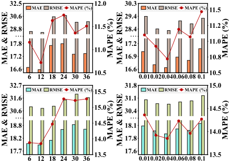
This section investigates the impact of two key hyperparameters on model performance: the patch operation length L and the regularization loss weight λ. As shown in Figure 4, L varies within the range [6, 12, 18, 24, 30, 36], with experiments conducted on the SD and GBA datasets as examples. We observe that when the patch length is too short, the model may lack sufficient expressive power due to its inability to capture long-term dependencies in the sequence. Conversely, when the patch length is too long, introducing redundant information (such as noise) leads to increased error across all metrics. Both datasets achieve optimal performance when L
is approximately 12. The right side of Figure 4 shows the sensitivity to the regularization loss weight λ. As λ increases from 0.01 to 0.04, all error metrics are significantly improved, demonstrating that moderate regularization is beneficial for model performance. However, when λ increases further, all metrics deteriorate notably.
4.5 Efficiency Comparison
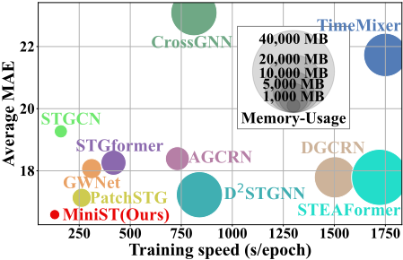
As shown in Figure 5, the training-efficiency comparison reveals a clear advantage for our model over more complex state-of-the-art baselines such as D2STGNN, DGCRN, and STEAFormer. Transformer-based frameworks suffer quadratic complexity in both spatial nodes and temporal steps, resulting in prohibitively high computational costs and limited scalability on large-scale traffic forecasting tasks. In contrast, MiniST strikes an optimal balance among prediction accuracy, training time, and memory consumption, making it a scalable yet efficient solution for both short- and long-term traffic prediction.
4.6 Performance on Extremely Large-scale Graph
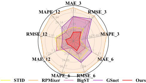
We further introduce a traffic network, City-Traffic-M, which comprises over 50,000 nodes. In this dataset, most existing models are unable to run due to memory constraints. We systematically compared the proposed model with several state-of-the-art methods. As shown in Figure 6, we report performance metrics for 3-step, 6-step, and 12-step forecasts, with results showing performance improvements of up to 6.14% by our model. This demonstrates the effectiveness of our compact model in extremely large-scale traffic networks.
4.7 Visualization and Analysis
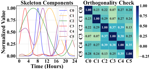
We visualize the learned basis components Xb in Figure 7. The results show that the model extracts B = 6 distinct basis components from the periodic data Xp. These components successfully capture fundamental urban traffic "rhythms," including bimodal commuting peaks, stable daytime flow patterns, and low-frequency nighttime activity, achieving substantial feature distillation from high-dimensional and highly redundant inputs. Meanwhile, the heatmap further validates the importance of the orthogonality loss. By minimizing the off-diagonal elements of the Grammatrix, the model enforces temporal decoupling among the basis vectors, ensuring their independence and diversity. This orthogonality constraint effectively prevents redundant pattern absorption and enhances expressive efficiency, allowing a minimal set of basis vectors to accurately represent complex spatiotemporal dynamics.
5 RelatedWork
5.1 Time Series Forecasting
In recent years, deep learning has achieved remarkable progress in time series forecasting [Ma et al., 2025c; Ma et al., 2025a]. Inspired by the success of Transformers, various Transformer-based models have been developed for this task. For instance, FEDformer [Zhou et al., 2022] enhances frequency-domain representations with Fourier and wavelet transforms to capture trends and seasonality with linear complexity, while PatchTST [Nie et al., 2022] adopts a patching strategy to preserve local temporal patterns and improve modeling efficiency. Meanwhile, MLP-based models have also shown competitive forecasting performance [Wang et al., 2024c; Zeng et al., 2023]. However, most existing methods mainly focus on temporal dependency modeling and fail to adequately capture spatial interactions among different sensors.
5.2 Spatiotemporal Graph Neural Network
Traffic forecasting is a core component of intelligent transportation systems [Wang et al., 2024a; Ma et al., 2025b; Zhang et al., 2023]. The dominant approaches in recent years have been spatiotemporal graph convolutional networks [Jiang and Luo, 2022; Jin et al., 2023]. For instance, STGCN [Yu et al., 2017] was among the first to integrate graph convolution with temporal convolution, enabling joint modeling of spatial and temporal dependencies. In recent years, several studies have incorporated the Transformer architecture into traffic forecasting, achieving superior performance. For example, D2STGNN [Shao et al., 2022b] employs a dual-stage graph learning strategy within a Transformer framework, separately modeling static and dynamic spatial dependencies. STGformer [Wang et al., 2024b] combines graph structure learning with self-attention mechanisms, effectively improving the modeling of long-range dependencies. Although spatiotemporal graph convolutional models have improved short-term forecasting accuracy, they often come with significantly increased parameter complexity. This poses a major limitation on their ability to handle long input sequences. In this work, we explore an extremely lightweight architecture that unlocks the potential of long-sequence modeling, aiming to improve both short-term and long-term forecasting performance.
6 Conclusion
In this paper, we explore performance gains by unlocking the input sequence length. We propose a minimalist spatiotemporal forecasting model that leverages an input backbone strategy and a pattern backbone strategy, encouraging the model to focus only on the most critical patterns and thereby reducing model complexity. Extensive experiments on multiple datasets demonstrate that our model achieves superior short-term and long-term traffic forecasting performance, along with outstanding computational efficiency.
Acknowledgements
This paper is partially supported by the National Natural Science Foundation of China (No.12227901) and the Natural Science Foundation of Jiangsu Province (BK20250482). The AI-driven experiments, simulations and model training were performed on the robotic AI-Scientist platform of Chinese Academy of Science.
@inproceedings{ijcai2026p298,
  title     = {MiniST: Unlocking Input Window Length in Traffic Flow Forecasting with Compact Parameters},
  author    = {Huang, Sheng and Wang, Guanjun and Ma, Jiaming and Wang, Binwu and Wang, Yang},
  booktitle = {Proceedings of the Thirty-Fifth International Joint Conference on
               Artificial Intelligence, {IJCAI-26}},
  publisher = {International Joint Conferences on Artificial Intelligence Organization},
  editor    = {Diego Calvanese},
  pages     = {2680--2688},
  year      = {2026},
  month     = {8},
  note      = {Main Track},
  doi       = {10.24963/ijcai.2026/298},
  url       = {https://doi.org/10.24963/ijcai.2026/298},
}
TY - CPAPER TI - MiniST: Unlocking Input Window Length in Traffic Flow Forecasting with Compact Parameters AU - Huang, Sheng AU - Wang, Guanjun AU - Ma, Jiaming AU - Wang, Binwu AU - Wang, Yang T2 - Proceedings of the Thirty-Fifth International Joint Conference on Artificial Intelligence, IJCAI-26 PB - International Joint Conferences on Artificial Intelligence Organization PY - 2026 SP - 2680 EP - 2688 DO - 10.24963/ijcai.2026/298 UR - https://doi.org/10.24963/ijcai.2026/298 ER -Copied
Machine-readable versions of this paper, for tools and AI agents:





