
History Doesn’t Repeat, but Its Patterns Echo: A Parallel Pairwise Negative-Sampling Framework for Temporal Link Prediction
Proceedings of the Thirty-Fifth International Joint Conference on Artificial Intelligence. Main Track. Pages 2717-2725.
https://doi.org/10.24963/ijcai.2026/302
Keywords
- Data Mining: Mining graphs
- Data Mining: Big data and scalability
- Data Mining: Parallel, distributed and cloud-based high performance mining
Abstract
Temporal link prediction with temporal graph neural networks (TGNNs) is increasingly used to model spatio-temporal dependencies in temporal graphs and to forecast future interactions among entities. Existing sampling-based training methods typically rely on random negative sampling and pointwise loss formulations, which often lead to suboptimal convergence and limited generalization due to low-quality negative samples. We propose ATNSF, a temporal graph learning framework with a hybrid negative sampling strategy that uses a portion of historical edges as hard negatives. For efficiency, we design an asynchronous parallel training pipeline for scalable optimization and introduce a pairwise sampled softmax loss that contrasts each positive instance with a batch of negatives to learn more discriminative representations. Finally, we theoretically show that jointly designing the loss function and negative sampling strategy is crucial for improving performance and generalization. Extensive experiments across six temporal graph datasets demonstrate that ATNSF improves the average AP from 0.724 to 0.827 (+0.103). Remarkably, it also accelerates training by 1.37× to 6.85×, achieving a 2.57× geometric mean speedup. The source code of this paper can be found at https://github.com/yongqiu-star/ATNSF.
- [Alvarez-Rodriguez et al., 2021] Unai Alvarez-Rodriguez, Federico Battiston, Guilherme Ferraz de Arruda, Yamir Moreno, Matjaž Perc, and Vito Latora. Evolutionary dynamics of higher-order interactions in social networks. Nature Human Behaviour, 5(5):586-595, 2021.
- [Bengio and Senecal, 2008] Yoshua Bengio and Jean- S Ébastien Senecal. Adaptive importance sampling to accelerate training of a neural probabilistic language model. IEEE Transactions on Neural Networks, 19(4):713-722, 2008.
- [Chang et al., 2020] Xiaofu Chang, Xuqin Liu, Jianfeng Wen, Shuang Li, Yanming Fang, Le Song, and Yuan Qi. Continuous-time dynamic graph learning via neural inter- action processes. In Proceedings of the 29th ACM Interna- tional Conference on Information & Knowledge Manage- ment, pages 145-154, 2020.
- [Chen et al., 2023] Changlu Chen, Yanbin Liu, Ling Chen, and Chengqi Zhang. Bidirectional spatial-temporal adap- tive transformer for urban traffic flow forecasting. IEEE Transactions on Neural Networks and Learning Systems, 34(10):6913-6925, 2023.
- [Chen et al., 2025] Ziyue Chen, Tongya Zheng, and Mingli Song. Curriculum negative mining for temporal networks. Neural Netw., 191(C), December 2025.
- [Cong et al., 2023] Weilin Cong, Si Zhang, Jian Kang, Baichuan Yuan, Hao Wu, Xin Zhou, Hanghang Tong, and Mehrdad Mahdavi. Do we really need complicated model architectures for temporal networks? In The Eleventh Inter- national Conference on Learning Representations, 2023.
- [Diaz-Aviles et al., 2012] Ernesto Diaz-Aviles, Lucas Dru- mond, Lars Schmidt-Thieme, and Wolfgang Nejdl. Real- time top-n recommendation in social streams. In Proceed- ings of the Sixth ACM Conference on Recommender Sys- tems, RecSys '12, page 59-66, New York, NY, USA, 2012. Association for Computing Machinery.
- [Gao et al., 2024] Kuang Gao, Chuang Liu, Jia Wu, Bo Du, and Wenbin Hu. Towards a better negative sampling strat- egy for dynamic graphs. Neural Netw., 173(C), May 2024.
- [Guo et al., 2019] Shengnan Guo, Youfang Lin, Ning Feng, Chao Song, and Huaiyu Wan. Attention based spatial- temporal graph convolutional networks for traffic flow fore- casting. In Proceedings of the AAAI conference on artificial intelligence, volume 33, pages 922-929, 2019.
- [He et al., 2024] Dongxiao He, Lianze Shan, Jitao Zhao, Hen- grui Zhang, Zhen Wang, and Weixiong Zhang. Exploitation of a latent mechanism in graph contrastive learning: Rep- resentation scattering. Advances in Neural Information Processing Systems, 37:115351-115376, 2024.
- [Huo et al., 2018] Zepeng Huo, Xiao Huang, and Xia Hu. Link prediction with personalized social influence. In Pro- ceedings of the AAAI conference on artificial intelligence, volume 32, 2018.
- [Jin et al., 2021] Di Jin, Zhizhi Yu, Pengfei Jiao, Shirui Pan, Dongxiao He, Jia Wu, Philip S Yu, and Weixiong Zhang. A survey of community detection approaches: From sta- tistical modeling to deep learning. IEEE Transactions on Knowledge and Data Engineering, 35(2):1149-1170, 2021.
- [Jin et al., 2024] Ming Jin, Huan Yee Koh, Qingsong Wen, Daniele Zambon, Cesare Alippi, Geoffrey I Webb, Irwin King, and Shirui Pan. A survey on graph neural networks for time series: Forecasting, classification, imputation, and anomaly detection. IEEE Transactions on Pattern Analysis and Machine Intelligence, 2024.
- [Kumar et al., 2019] Srijan Kumar, Xikun Zhang, and Jure Leskovec. Predicting dynamic embedding trajectory in tem- poral interaction networks. In Proceedings of the 25th ACM SIGKDD international conference on knowledge discovery & data mining, pages 1269-1278, 2019.
- [Li et al., 2013] Xirong Li, CeesG. M. Snoek, Marcel Wor- ring, Dennis Koelma, and Arnold W. M. Smeulders. Boot- strapping visual categorization with relevant negatives. IEEE Transactions on Multimedia, 15(4):933-945, 2013.
- [Li et al., 2025] Yingxuan Li, Yuanyuan Xu, Xuemin Lin, Wenjie Zhang, and Ying Zhang. Ranking on dynamic graphs: An effective and robust band-pass disentangled approach. In Proceedings of the ACM Web Conference, 2025.
- [Lu et al., 2024] Xiaodong Lu, Leilei Sun, Tongyu Zhu, and Weifeng Lv. Improving temporal link prediction via tem- poral walk matrix projection. In The Thirty-eighth Annual Conference on Neural Information Processing Systems, 2024.
- [Luo and Li, 2022] Yuhong Luo and Pan Li. Neighborhood- aware scalable temporal network representation learning. In Bastian Rieck and Razvan Pascanu, editors, Proceedings of the First Learning on Graphs Conference, volume 198 of Proceedings of Machine Learning Research, pages 1:1- 1:18. PMLR, 09-12 Dec 2022.
- [Mao et al., 2021] Xin Mao, Wenting Wang, Yuanbin Wu, and Man Lan. Boosting the speed of entity alignment 10 ×: Dual attention matching network with normalized hard sample mining. In Proceedings of the Web Conference 2021, WWW '21, page 821-832, New York, NY, USA, 2021. Association for Computing Machinery.
- [Noh et al., 2018] Junhyug Noh, Soochan Lee, Beomsu Kim, and Gunhee Kim. Improving occlusion and hard nega- tive handling for single-stage pedestrian detectors. In Pro- ceedings of the IEEE Conference on Computer Vision and Pattern Recognition (CVPR), June 2018.
- [Pareja et al., 2020] Aldo Pareja, Giacomo Domeniconi, Jie Chen, Tengfei Ma, Toyotaro Suzumura, Hiroki Kanezashi, Tim Kaler, Tao Schardl, and Charles Leiserson. Evolvegcn: Evolving graph convolutional networks for dynamic graphs. In Proceedings of the AAAI conference on artificial intelli- gence, volume 34, pages 5363-5370, 2020.
- [Poursafaei et al., 2022] Farimah Poursafaei, Shenyang Huang, Kellin Pelrine, and Reihaneh Rabbany. Towards better evaluation for dynamic link prediction. Advances in Neural Information Processing Systems, 35:32928-32941, 2022.
- [Qin et al., 2021] Xiao Qin, Nasrullah Sheikh, Berthold Rein- wald, and Lingfei Wu. Relation-aware graph attention model with adaptive self-adversarial training. Proceed- ings of the AAAI Conference on Artificial Intelligence, 35(11):9368-9376, May 2021.
- [Rao et al., 2016] Jinfeng Rao, Hua He, and Jimmy Lin. Noise-contrastive estimation for answer selection with deep neural networks. In Proceedings of the 25th ACM Inter- national on Conference on Information and Knowledge Management, CIKM '16, page 1913-1916, New York, NY, USA, 2016. Association for Computing Machinery.
- [Rendle and Freudenthaler, 2014] Steffen Rendle and Christoph Freudenthaler. Improving pairwise learning for item recommendation from implicit feedback. In Proceedings of the 7th ACM International Conference on Web Search and Data Mining, WSDM '14, page 273-282, New York, NY, USA, 2014. Association for Computing Machinery.
- [Rendle et al., 2009] Steffen Rendle, Christoph Freuden- thaler, Zeno Gantner, and Lars Schmidt-Thieme. Bpr: Bayesian personalized ranking from implicit feedback. In Proceedings of the Twenty-Fifth Conference on Uncertainty in Artificial Intelligence, UAI '09, page 452-461, Arlington, Virginia, USA, 2009. AUAI Press.
- [Rossi et al., 2020] Emanuele Rossi, Ben Chamberlain, Fab- rizio Frasca, Davide Eynard, Federico Monti, and Michael Bronstein. Temporal graph networks for deep learning on dynamic graphs. In ICML 2020 Workshop on Graph Representation Learning, 2020.
- [Song et al., 2019] Weiping Song, Zhiping Xiao, Yifan Wang, Laurent Charlin, Ming Zhang, and Jian Tang. Session- based social recommendation via dynamic graph attention networks. In Proceedings of the Twelfth ACM international conference on web search and data mining, pages 555-563, 2019.
- [Sun et al., 2019] Qianru Sun, Yaoyao Liu, Tat-Seng Chua, and Bernt Schiele. Meta-transfer learning for few-shot learning. In Proceedings of the IEEE/CVF Conference on Computer Vision and Pattern Recognition (CVPR), June 2019.
- [Wang et al., 2020] Yanbang Wang, Yen-Yu Chang, Yunyu Liu, Jure Leskovec, and Pan Li. Inductive representation learning in temporal networks via causal anonymous walks. In International Conference on Learning Representations, 2020.
- [Wang et al., 2021a] Lu Wang, Xiaofu Chang, Shuang Li, Yunfei Chu, Hui Li, Wei Zhang, Xiaofeng He, Le Song, Jingren Zhou, and Hongxia Yang. TCL: transformer-based dynamic graph modelling via contrastive learning. CoRR, abs/2105.07944, 2021.
- [Wang et al., 2021b] Xuhong Wang, Ding Lyu, Mengjian Li, Yang Xia, Qi Yang, Xinwen Wang, Xinguang Wang, Ping Cui, Yupu Yang, Bowen Sun, et al. Apan: Asynchronous propagation attention network for real-time temporal graph embedding. In Proceedings of the 2021 international con- ference on management of data, pages 2628-2638, 2021.
- [Wang et al., 2023] Wen Wang, Wei Zhang, Shukai Liu, Qi Liu, Bo Zhang, Leyu Lin, and Hongyuan Zha. Incor- porating link prediction into multi-relational item graph modeling for session-based recommendation. IEEE Trans- actions on Knowledge and Data Engineering, 35(3):2683- 2696, 2023.
- [Wang et al., 2024] Luzhi Wang, Dongxiao He, He Zhang, Yixin Liu, Wenjie Wang, Shirui Pan, Di Jin, and Tat-Seng Chua. Goodat: Towards test-time graph out-of-distribution detection. In Proceedings of the AAAI Conference on Arti- ficial Intelligence, volume 38, pages 15537-15545, 2024.
- [Wu et al., 2019] Zonghan Wu, Shirui Pan, Guodong Long, Jing Jiang, and Chengqi Zhang. Graph wavenet for deep spatial-temporal graph modeling. In Proceedings of the Twenty-Eighth International Joint Conference on Artificial Intelligence, IJCAI 2019, Macao, China, August 10-16, 2019, pages 1907-1913. ijcai.org, 2019. IJCAI
- [Wu et al., 2020] Zonghan Wu, Shirui Pan, Guodong Long, Jing Jiang, Xiaojun Chang, and Chengqi Zhang. Connect- ing the dots: Multivariate time series forecasting with graph neural networks. In Proceedings of the 26th ACM SIGKDD international conference on knowledge discovery & data mining, pages 753-763, 2020.
- [Wu et al., 2021] Zonghan Wu, Shirui Pan, Fengwen Chen, Guodong Long, Chengqi Zhang, and Philip S Yu. A com- prehensive survey on graph neural networks. IEEE transac- tions on neural networks and learning systems, 32(1):4-24, 2021.
- [Wu et al., 2024] Jiancan Wu, Xiang Wang, Xingyu Gao, Ji- awei Chen, Hongcheng Fu, and Tianyu Qiu. On the effec- tiveness of sampled softmax loss for item recommendation. ACM Transactions on Information Systems, 42(4):1-26, 2024.
- [Xu et al., 2020] Da Xu, Chuanwei Ruan, Evren Korpeoglu, Sushant Kumar, and Kannan Achan. Inductive representa- tion learning on temporal graphs. In International Confer- ence on Learning Representations, 2020.
- [Xu et al., 2024] Yuanyuan Xu, Wenjie Zhang, Ying Zhang, Maria E. Orlowska, and Xuemin Lin. Timesgn: Scalable and effective temporal graph neural network. In Proceed- ings of the IEEE International Conference on Data Engi- neering, pages 3297-3310, 2024.
- [Yu et al., 2021] Le Yu, Bowen Du, Xiao Hu, Leilei Sun, Liangzhe Han, and Weifeng Lv. Deep spatio-temporal graph convolutional network for traffic accident prediction. Neurocomputing, 423:135-147, 2021.
- [Yu et al., 2023] Le Yu, Leilei Sun, Bowen Du, and Weifeng Lv. Towards better dynamic graph learning: New architec- ture and unified library. Advances in Neural Information Processing Systems, 36, 2023.
- [Zhang et al., 2013] Weinan Zhang, Tianqi Chen, Jun Wang, and Yong Yu. Optimizing top-n collaborative filtering via dynamic negative item sampling. In Proceedings of the 36th International ACM SIGIR Conference on Research and Development in Information Retrieval, SIGIR '13, page 785-788, 2013.
References were extracted automatically from the PDF and may contain errors.
Full text extracted automatically from the PDF; figures, tables and equations may differ. The PDF is the version of record.
1 Introduction
Temporal graph modeling provides a flexible representation of real-world scenarios by abstracting entities as nodes and the dynamic, time-varying interactions or relationships between these entities as temporal edges [Wu et al., 2021; Jin et al., 2024]. This framework is widely applicable to various domains, such as social networks [Huo et al., 2018; Kumar et al., 2019; Alvarez-Rodriguez et al., 2021], traffic networks [Chen et al., 2023; Wu et al., 2019; Guo et al., 2019; Yu et al., 2021], recommendation systems [Jin et al., 2021;
∗Corresponding author.
Song et al., 2019; Wang et al., 2023], and financial transactions [Wang et al., 2021b; Wu et al., 2020]. Accurate prediction of future links enables a deeper understanding of the evolutionary patterns of dynamic networks. Recent advances in temporal graph neural networks have significantly improved temporal link prediction[Jin et al., 2024; Wang et al., 2024]. Current methods leverage temporal encoding[Chen et al., 2023; Wu et al., 2020; He et al., 2024] and attention mechanisms[Xu et al., 2020; Wang et al., 2021a; Yu et al., 2023] to model fine-grained temporal dependencies and adopt temporal walk-based techniques[Wang et al., 2020; Lu et al., 2024] to capture higher-order structural patterns over time.
Although these approaches achieve strong empirical performance, their accuracy often degrades under specific data distributions, particularly in sparse or rapidly evolving graphs. This limitation suggests that current training strategies may restrict the robustness and generalization of the model. Existing methods treat the task as binary classification and use random negative sampling with pointwise losses such as binary cross-entropy (BCE). Temporal link prediction aims to forecast future interactions between node pairs based on past observations, but only realized interactions are recorded and non-existent edges are never explicitly observed. As a result, current TGNN-based methods generate negatives by randomly sampling node pairs without observed interactions.
However, integrating Negative sampler modules into TGNN training introduces significant efficiency challenges and three fundamental drawbacks. First, negative sampling accuracy is limited by commonly used random negative sampling (RNS) strategies, which worsen the mislabeled-sample problem by producing negative samples that lack meaningful contrast, especially in complex contexts such as historical and inductive link prediction [Poursafaei et al., 2022; Wang et al., 2024]. A major challenge is the prevalence of false negatives in dense graphs, where positive links are mistakenly labeled as negative. These incorrect labels mislead the model and reduce accuracy, particularly in graphs with complex temporal-topological dynamics. Second, sampling-based training efficiency is constrained by recent temporal training paradigms, which impose strict temporal dependencies across sequentially sampled mini-batches because evolving states such as node memory are updated on a per-batch basis. Consequently, the computation associated with each mini-batch must adhere to the node states produced by the preceding mini-batches, making it difficult to eliminate or decouple these temporal cross-batch overlap dependencies. Third, temporal model generalization is limited by pointwise loss functions such as binary cross-entropy. By considering positive and negative samples independently and with equal weight, pointwise loss functions are unable to effectively capture the relative significance and relationships between sparse positive instances and dense negative ones, resulting in suboptimal convergence and inadequate generalization performance.
To address these issues, we propose ATNSF, an Accurate Temporal Negative Sampling Framework, which incorporates a novel hierarchical-level negative sampling strategy and pairwise loss enhancement module, designed explicitly from a ranking perspective. First, to address the challenge of negative sampling accuracy (Bottleneck 1), we propose a hybrid sampling methodology that augments conventional negative sampling with a metric-guided, balanced proportion of hard negatives during training. Selected from historical interactions to deliberately confound the model, these instances provide a clear quantitative contrast to positives, improving the model's ability to learn discriminative representations. This approach reduces false positives caused by purely random sampling, which often yields semantically similar or weakly informative negatives. Second, to improve the efficiency of negative sampling-based TGNN training (Bottleneck 2), we introduce a memory-backed, asynchronous, parallel training pipeline that uses dedicated sampling memory and decouples sampling from training. ATNFS employs a unified streaming pipeline with operators organized in a bounded queue, where temporal neighbor sampling, negative edge sampling, and feature construction run sequentially before the mini-batch is enqueued. A worker thread continuously prepares the upcoming batches in the background, ensuring a steady supply of preprocessed data for training. Third, to improve temporal model generalization (Bottleneck 3), we propose a pairwise softmax loss tailored for predicting future temporal links. This loss maintains the relative scores between each positive sample and a batch of negatives, ensuring the positive score exceeds the negatives. It effectively leverages generated negatives, reducing false negatives from mislabeled low-probability samples and enhancing the model's ability to distinguish subtle differences in difficult sample pairs.
Theoretically, we reveal that the softmax loss function is particularly well-suited for learning from the hard negative samples introduced by our hybrid strategy, further enhancing model performance. Our comprehensive experiments on six temporal graph datasets demonstrate that ATNSF achieves significant improvements in both accuracy and efficiency, increasing the average AP from 0.724 to 0.827 (+0.103) and accelerating training by 1.37×-6.85× (geo-mean 2.57×).
2 RelatedWork
2.1 Temporal Graph Learning
Temporal graph learning (TGL) aims to predict future interactions between nodes based on historical topological information [Jin et al., 2024; He et al., 2024]. Early models in this field treated the temporal graph as a sequence of snapshots and applied GNNs for prediction, such as Evolvegcn [Pareja et al., 2020]. These models fall into the category of discrete-time temporal graph learning approaches. Recently, temporal graphs have increasingly been modeled as sequences of time-dependent interactions, known as continuous-time temporal graph learning[Chang et al., 2020]. A main advance is updating node states using temporal information, as in JODIE [Kumar et al., 2019], which employs an RNN to capture temporal dynamics. Another major direction models both topology and time from historical graphs, exemplified by TGAT [Xu et al., 2020], which uses self-attention to aggregate multi-hop neighborhood information. Graph-based methods that aggregate node and edge relations have also emerged, such as GraphMixer [Cong et al., 2023], which uses an MLPMixer to aggregate first-order neighbors and edges. A further advance is the combination of intermediate node states with neighborhood information, as in TGN [Rossi et al., 2020], which jointly updates node states and aggregates neighborhoods to better model temporal relationships. Recent studies show that incorporating pairwise node information improves performance. DyGFormer [Yu et al., 2023] extracts neighborhood co-occurrence information and combines it with a transformer for feature mixing, while NAT [Luo and Li, 2022] decodes pairwise information via a dictionary-style neighborhood representation. TPNet [Lu et al., 2024] is another example, injecting pairwise information through matrix operations. Recent complementary work further studies scalability and ranking-oriented objectives: TimeSGN [Xu et al., 2024] improves temporal message passing with a divided temporal message passing paradigm, while BandRank [Li et al., 2025] targets dynamic graph ranking through band-pass disentangled representations and a harmonic ranking loss.
2.2 Temporal Negative Sampling
Negative sampling constructs negative instances for observed positives and is widely used to improve training efficiency and ranking quality. The simplest strategy is random negative sampling [Rendle et al., 2009; Diaz-Aviles et al., 2012]; in TGL, it commonly forms (u, vneg, t) by randomly choosing vneg ∈ V for a positive edge (u, v, t). This strategy is efficient but insensitive to temporal structure, making it unlikely to select informative negatives. Hard or adaptive negative sampling has therefore been studied in image classification [Li et al., 2013; Sun et al., 2019], object detection [Noh et al., 2018], NLP [Bengio and Senecal, 2008; Rao et al., 2016], recommendation [Zhang et al., 2013; Rendle and Freudenthaler, 2014], and knowledge graphs [Mao et al., 2021; Qin et al., 2021]. Pairwise ranking and sampled-softmax objectives are also common in recommendation [Rendle et al., 2009; Rendle and Freudenthaler, 2014; Wu et al., 2024].
These static or recommendation-oriented methods inspire our design, but they do not directly address chronological constraints in temporal link prediction. Recent temporal studies improve negative sampling for dynamic graphs [Gao et al., 2024; Chen et al., 2025], and Poursafaei et al. [Poursafaei et al., 2022] show that models struggle under historical and inductive test-time negative sampling, especially on reoccurring edges. Different from settings where historical or reoccurring edges are mainly used to stress-test evaluation, ATNSF injects only past interactions before the current batch as trainingtime hard negatives. We further combine this temporal hybrid sampler with a pairwise sampled-softmax loss, improving robustness to false negatives while preserving random negatives for generalization.
3 Preliminaries
Definition 1 (Temporal Graph). A temporal graph is defined as a tuple G = (V, E,Xv,Xe), where V represents the set of nodes, and each node u ∈ V is associated with a feature vector xu ∈ RdV . The set of temporal edges is denoted by E ⊆ V × V × Z, where each edge is represented as a triplet (ui, vi, ti), with ui, vi ∈ V indicating the source and target nodes, respectively, and ti ∈ Z representing the integer timestamp of the i-th interaction. The timestamps are assumed to follow a non-decreasing order, i.e., t1 ≤ t2 ≤ · · · ≤ ti ≤ · · · ≤ tlatest, where tlatest is the latest timestamp of the observed period. Each edge e ∈ E is further endowed with a feature vector xe ∈ RdE . The node feature set and edge feature set are denoted by Xv = {xu | u ∈ V} and Xe = {xe | e ∈ E}, respectively. If the temporal graph does not include explicit node or edge features, these features are initialized as null vectors, i.e., xu = 0 ∈ RdV for all u ∈ V, and xe = 0 ∈ RdE for all e ∈ E.
Temporal Graph Link Prediction Task. Given a temporal graph G = (V, E,Xv,Xe), the task of temporal graph link prediction is to predict the likelihood of the existence of a future edge (u, v, t), where u ∈ V, v ∈ V, and t > T , based on the information contained in G.
Temporal Negative Sampling. Given a continuous dynamic graph G = (V, E), the set of all possible negative samples is defined as Epossible = {(ui, vi, ti) | ui, vi ∈ V, (ui, vi, ti) /∈ E, 0 ≤ ti ≤ tlatest}. A negative sampling strategy refers to a method for selecting a subset Eneg ⊆ Epossible to be used during training.
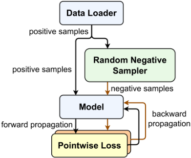
Figure 1 illustrates that a standard TGNN training procedure begins with the data loader, which provides positive samples extracted from the temporal graph. A random negative sampler is then used to generate the corresponding negative samples. Both positive and negative samples are fed into the model for forward propagation, where the model processes the inputs to produce predictions. A pointwise loss function is used to compute the difference between the predictions and the ground truth labels for each sample. Based on the computed loss, the model parameters are updated through backward propagation, iteratively refining the model performance.
4 Re-evaluating TGNN Training Framework
In this section, we first describe the standard training procedure for temporal graph neural networks, highlighting the roles of negative sampling and the loss function. We then show how existing methods suffer from sample homogeneity and false negatives, leading to false positives and false negatives. Two novel findings are derived from our re-evaluation of the TGNN training framework.
4.1 Lack of Robustness and Efficiency to Sampler-Based Training Methodology
The random negative sampler takes as input a batch of positive samples (u, v, t) and generates a batch of negative samples (u, vneg, t) by randomly sampling a set of destination nodes vneg of size batch size from the set of nodes V. The most significant advantage of such random negative sampling is its efficiency as it avoids computationally expensive procedures while enabling easy differentiation between positive samples and some straightforward negative samples. However, research indicates that models trained this way tend to perform poorly on challenging negative edges, such as historical edges and inductive edges [Poursafaei et al., 2022], showing a higher frequency of false positives (FP issues). The underlying cause lies in the inherent simplicity of the random sampling method, which is insufficient to capture the complexity of rare and challenging examples within the vast sample space. Furthermore, due to sampling efficiency considerations, the current random sampling technique does not perform conflict checks on positive samples within a batch, resulting in some samples being simultaneously labeled both positive and negative [Poursafaei et al., 2022]. Another issue arises from data collection, where certain positive samples may be missed, resulting in misclassification of some positive samples as negative. Although these occurrences are infrequent, they still contribute to the degradation of training performance, exacerbating the false negative (FN) issue.
Observation I: Achieving an effective and efficient hard negative sampler is necessary, which is not only to improve the performance but also to impact the entire training pipeline.
4.2 Insensitivity of Loss Function to Individual Samples
Recent work on TGNNs employs a pointwise loss function instantiated as the binary cross-entropy (BCE) loss, which is defined as follows:
where N is the total number of samples, yi ∈ {0, 1} represents the ground truth label, and pi is the predicted probability that the i-th sample is a positive sample. Binary Cross-Entropy (BCE) loss is widely employed in binary classification tasks because it forces both positive and negative instances to contribute comparably to the optimization process. However, this property simultaneously increases the sensitivity of TGNN models to the quality of negative samples. In particular, false negative instances are especially challenging to identify and remove, and their presence can introduce bias into the TGNN model training procedure.
Observation II: Pointwise loss impacts the generalization of temporal prediction, which cannot adapt to natural sample distributions.
5 Methodology
In this section, we propose a hybrid sampling strategy, jointly optimized in an asynchronous training pipeline with a powerful pairwise loss to address these issues and theoretically prove their effectiveness for temporal link prediction.
5.1 Hybrid SamplingMethodology
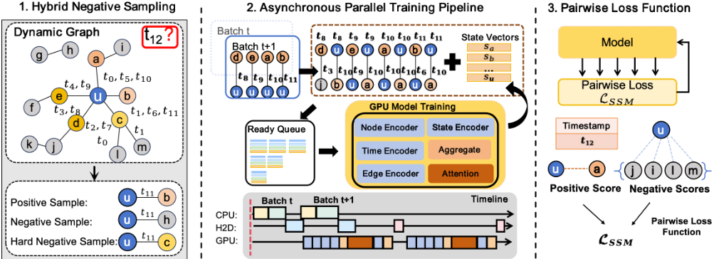
Building on our observations, we propose an enhanced hybrid negative sampling method (Figure 2) that integrates random and hard negative sampling. To mitigate the FP issue caused by the simplicity of the random negative sampling approach, we introduce historical edges, which commonly perform poorly in current models, as hard negative samples during training. Furthermore, we incorporate a parameter γ to regulate the balance between easy and hard samples, where γ ∈ [0, 1]
represents the proportion of easy samples. In our implementation, we use batch-based training as described in Algorithm 1, where the input consists of the temporal graph G = {V, E}, a batch of positive edges Ebp, and a balancing parameter γ. The algorithm first extracts the global earliest timestamp t0 from E. From the mini-batch Ebp, it obtains the batch size l = |Ebp| and the associated timestamp sequence T = [t1, t2, . . . , tl] for subsequent assignment. Random negative samples are drawn from all possible node pairs, excluding E ′bp , while historical negative samples are extracted from edges with timestamps between t0 and t1. The set of hard negatives is created by removing E ′bp from the historical set. Using the balancing parameter γ, a proportion of random negatives and historical negatives is selected, with the final batch of negative samples assigned timestamps and returned for training. This hybrid negative sampling strategy improves the model's performance by allowing it to effectively handle both simple and challenging samples.
5.2 Asynchronous Parallel Training Pipeline
Temporal graph training enforces strict chronological dependencies across mini-batches, since the evolving state (e.g., node memory) updated by batch Bt must be consumed by Bt+1. To maximize resource utilization without violating dependencies, we propose an asynchronous parallel TGNN training pipeline that concurrently overlaps CPU-based sample preprocessing with GPU-resident computation. Specifically, a dedicated CPU worker continuously prepares subsequent minibatches by performing temporal neighbor sampling, negative edge sampling, and feature construction, and subsequently enqueues the processed batches into a bounded ready queue. Concurrently, the training process dequeues batches from the ready queue in a first-in, first-out manner and performs forward and backward optimizations, as well as parameter updates, strictly following the temporal order of samples. To reduce host-side overhead, we allocate a fixed pool of reusable,
Input: G = (V, E), Ebp, γ Output: Eneg 1 t0 ←min{t | (·, ·, t) ∈ E} 2 l ← |Ebp| 3 T ← [t1, t2, . . . , tl] from Ebp 4 E ′bp ← {(ui, vi)}li=1 from Ebp 5 E ′pos ←V ×V // all possible node pairs 6 E ′ rand ← E ′pos \ E ′bp 7 E ′hist ← {(u, v) | (u, v, t) ∈ E, t0 ≤ t < t1} 8 E ′hard ← E ′hist \ E ′bp 9 E ′neg ← ∅ 10 E ′neg ← E ′neg ∪ Sample(E ′ rand , ⌈lγ⌉) 11 E ′neg ← E ′neg ∪ Sample(E ′hard , ⌈l(1 - γ)⌉) 12 Eneg ← ∅; idx ← 1 13 foreach (u, v) ∈ E ′neg do 14 Eneg ← Eneg ∪ {(u, v, T[idx])} 15 idx ← idx + 1 16 return Enegmemory-backed host buffers and store prepared tensors in pinned host memory for low-latency GPU transfers.
Let TPREP denote the CPU-side preprocessing time (including neighbor retrieval and negative sampling), TH2D the host-to-device data transfer time, and TGPU the GPU computation time. The total time per iteration in the sequential (non-pipelined) setting is therefore
whereas, under our steady-state pipelined execution, the periteration latency becomes
indicating that the preprocessing overhead can be fully hidden when TGPU ≥ TPREP + TH2D. Furthermore, we encapsulate the negative sampling in a modular plug-in operator N(·), enabling diverse strategies (e.g., uniform random negatives or those from historical interactions) without modifying the core training loop.
5.3 Pairwise Loss Function
To mitigate the issue of false negatives that arise from label noise introduced during the negative sampling procedure, we deliberately avoid casting the prediction task as a conventional binary classification problem[Wu et al., 2024]. Instead, we propose a pairwise sampled softmax (SSM) loss, which, to the best of our knowledge, constitutes the first instantiation of a pairwise loss function within the context of temporal graph link prediction. This proposed methodology prioritizes assigning higher predicted probabilities for positive samples relative to their corresponding negative samples, thereby mitigating the adverse effects of potential mislabeling during negative sampling. By adopting a pairwise learning paradigm, our method enables the model to learn the relative ranking between positive and negative samples, instead of evaluating each sample in isolation. Consequently, positive samples are more likely to be assigned higher predictive probabilities, while negative samples are systematically penalized, which collectively enhances the model's capacity to produce more accurate predictions.
Specifically, the corresponding loss function for temporal graph link prediction can be written as:
In this formulation, f(ui, vi, ti) represents the predicted score for a positive sample (ui, vi, ti), where ui, vi ∈ V and ti ∈ Z. The term f(uj, vj, tj) corresponds to the predicted scores for the negative samples, which are drawn from the negative sample distribution N. The loss function is designed to maximize the predicted score for positive samples while simultaneously minimizing the predicted scores for negative samples. This ensures that the model assigns a higher probability to the correct links, thus improving its predictive accuracy. The exponential function applied to the predicted scores amplifies the difference between positive and negative samples, and the negative logarithm ensures effective minimization during training, stabilizing the learning process.
5.4 Complexity and Theoretical Analysis
In this section, we address two key questions. First, we discuss the complexity of the negative sampling strategy. Compared to the original approach, our method introduces additional costs for constructing the sets Epos and Ehist, which have complexities of O(|N|2 ) and O(|E|), respectively. Furthermore, the difference operation to detect conflicts with positive samples can be optimized to O(1) complexity by using hash tables. In the case of large-scale datasets, GPU-based parallelization strategies could be explored to accelerate the process, while preprocessing steps offer additional opportunities to further speed up the training. These optimizations represent important areas for future research to enhance the efficiency of our approach.
Secondly, we examine whether our loss function effectively enhances the model's ability to learn from hard negative samples. Following the work by Wu et al. [Wu et al., 2024], we compute the derivative of the loss function with respect to f(uk, vk, tk), and by setting the derivative equal to zero, we obtain the nearly closed-form solution of f(uk, vk, tk) :
In this equation, f(uk, vk, tk) represents the predicted score of the sample (uk, vk, tk), and pn(k) denotes the probability of selecting a negative sample from the distribution pn. The termN is the total number of negative samples, and E refers to the set of all edges in the temporal graph. The expression above shows that f ∗ (uk, vk, tk) is inversely related to pn(k), meaning that as the likelihood of selecting a negative sample increases, the corresponding value of f ∗ (uk, vk, tk) decreases.
This result shows that increasing the probability of selecting hard negative samples, which are more challenging to classify, helps the model to focus on these difficult examples and better distinguish true positives from hard negatives, improving temporal graph link prediction performance.
| Dataset | Model | Accuracy (AP) | Efficiency (Time) | |||||||
|---|---|---|---|---|---|---|---|---|---|---|
| RNS | ENS† | CurNM† | ATNSF | ∆ | RNS (s) | ATNSF (s) | Speedup (×) | |||
| Wiki JODIE | 0.704 | 0.786 | 0.803 - | 0.786 0.894 | -0.017 | 0.95 | 0.43 2.46 | 2.21 1.37 1.86 | ||
| TGAT | 0.838 | 0.832 | 0.056 | 3.38 | ||||||
| TGN | 0.882 | 0.908 | 0.921 | 0.901 | -0.020 | 5.36 | 2.88 | |||
| 0.682 | 0.677 | 0.657 | 0.873 | |||||||
| MOOC JODIE TGAT | 0.745 | - | - | 0.956 | 0.191 0.211 | 2.09 10.39 | 0.93 5.22 | 2.25 1.99 | ||
| TGN | 0.755 | 0.772 | 0.782 | 0.968 | 0.186 | 19.88 | 6.48 | 3.07 | ||
| JODIE | 0.667 | 0.834 | 0.835 | 0.792 | -0.043 | 4.05 | 1.47 | 2.76 | ||
| REDDIT TGAT | 0.675 | 0.809 | - | 0.762 | -0.047 | 20.53 | 9.86 | 2.08 | ||
| TGN | 0.678 | 0.890 | 0.881 | 0.780 | -0.110 | 79.09 | 11.54 | 6.85 | ||
| JODIE | 0.653 | 0.552 | 0.570 | 0.684 | 0.031 | 7.30 | 2.67 | 2.73 | ||
| LastFM TGAT | 0.700 | - | - | 0.731 | 0.031 | 30.44 | 16.19 | 1.88 | ||
| TGN | 0.706 | 0.740 | 0.716 | 0.798 | 0.058 | 105.77 | 19.83 | 5.33 | ||
| Avg. / GeoMean | Win/Tie/Lose | 0.724 7 / 0 / | 0.780 (vs. best | 0.771 baseline) | 0.827 | +0.044 | - | - | 2.57 | |
6 Experiments
6.1 Experimental Settings
Main Setup. Our main experiments are conducted under the TGL training pipeline, which provides an efficient and unified implementation for temporal link prediction. We evaluate negative sampling strategies on four benchmark datasets: Wikipedia, Reddit, MOOC, and LastFM, using three temporal backbones (JODIE, TGN, and TGAT). The main comparison focuses on negative sampling strategies. We compare our method ATNSF with Random Negative Sampling (RNS) and two representative baselines, ENS [Gao et al., 2024] and CurNM [Chen et al., 2025]. To ensure fairness, RNS and ATNSF are reproduced within the same TGL pipeline under identical experimental configurations, including dataset splits, evaluation protocol, backbone architectures, and hyperparameters. For ENS and CurNM, we cite the reported results from the original papers (marked with † ), since their released artifacts are not directly runnable in our environment; we follow the evaluation protocol specified in these works.
Metrics and Efficiency. We adopt Average Precision (AP) as the primary metric for the main comparison. In addition, we report training efficiency measured by wall-clock training time (seconds per epoch) and compute speedup relative to RNS. Efficiency is evaluated only between RNS and ATNSF within the same TGL pipeline, ensuring that the speedup reflects the impact of our sampling design rather than differences across training frameworks.
Implementation Details. All methods are trained using Adam with early stopping (patience = 20), selecting the best checkpoint based on validation performance. Unless otherwise specified, we use a learning rate of 1e-4 and a batch size of 200. Experiments are conducted on an Ubuntu server equipped with an Intel Xeon Platinum 8375C CPU (128 cores) and 4 NVIDIA RTX 4090 GPUs (24GB each).
6.2 Comparison with TGNN Frameworks
Table 1 summarizes the accuracy-efficiency trade-off. ATNSF is competitive across datasets and backbones, with the largest gains on MOOC: it improves JODIE from 0.682 (RNS) to 0.873 (+0.191 AP) and TGN from 0.782 (CurNM) to 0.968 (+0.186 AP). Although ATNSF is not the top AP method in every dataset-backbone pair, it achieves the best average AP in Table 1. It also reduces training time by 1.37×-6.85×, with a 2.57× geometric-mean speedup over RNS. These results show that temporally aware hard negatives are effective for recurrent temporal dependencies while preserving efficient training. The mixed per-dataset behavior further suggests that ATNSF prioritizes a stable accuracy-efficiency trade-off rather than winning every individual dataset-backbone pair.
6.3 Robustness Under Test-time Distribution Shifts
To evaluate robustness under test-time distribution shifts, we study TPNet [Lu et al., 2024] within DyGLib [Yu et al., 2023] using the EdgeBank [Poursafaei et al., 2022] rnd, hist, and ind protocols. We report AUC-ROC (×100) in transductive and inductive settings.
Table 2 shows that the baseline remains strong under rnd but degrades under hist and ind, whereas ATNSF improves most challenging settings with only minor rnd changes. The largest gains appear on Wikipedia and Reddit under inductive hist/ind evaluation, supporting our motivation that temporally plausible negatives are harder and more informative.
6.4 Detailed Analysis
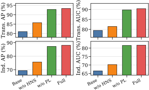
Ablation Study. We evaluate four Wikipedia configurations under historical transductive and inductive protocols: the full method, variants without HNS or PL, and the standard baseline.
| Data/NSS | Trans. | Ind. | ||||
|---|---|---|---|---|---|---|
| Base | Ours | Imp. | Base | Ours | Imp. | |
| Wiki-rnd | 99.28 | 99.31 | +0.03 | 98.83 | 98.89 | +0.06 |
| Wiki-hist | 79.46 | 90.39 | +10.9 | 66.51 | 81.72 | +15.2 |
| Wiki-ind | 75.88 | 85.27 | +9.39 | 66.51 | 81.72 | +15.2 |
| Reddit-rnd | 99.22 | 99.20 | -0.02 | 98.72 | 98.70 | -0.02 |
| Reddit-hist | 82.20 | 86.85 | +4.65 | 62.71 | 70.13 | +7.42 |
| Reddit-ind | 82.09 | 85.10 | +3.01 | 62.70 | 70.13 | +7.43 |
| MOOC-rnd | 96.86 | 96.76 | -0.10 | 96.62 | 96.41 | -0.21 |
| MOOC-hist | 92.80 | 94.01 | +1.21 | 86.61 | 88.45 | +1.84 |
| MOOC-ind | 87.87 | 89.06 | +1.19 | 86.62 | 88.45 | +1.83 |
| Enron-rnd | 94.05 | 94.12 | +0.07 | 90.67 | 91.00 | +0.33 |
| Enron-hist | 80.73 | 82.77 | +2.04 | 70.23 | 72.61 | +2.38 |
| Enron-ind | 74.35 | 77.57 | +3.22 | 70.23 | 72.61 | +2.38 |
| UCI-rnd | 96.76 | 96.34 | -0.42 | 94.38 | 94.23 | -0.15 |
| UCI-hist | 80.34 | 83.35 | +3.01 | 71.06 | 77.11 | +6.05 |
| UCI-ind | 70.61 | 76.39 | +5.78 | 71.08 | 77.12 | +6.04 |
| Can.-rnd | 88.85 | 90.53 | +1.68 | 69.20 | 72.08 | +2.88 |
| Can.-hist | 85.27 | 92.36 | +7.09 | 70.61 | 72.85 | +2.24 |
| Can.-ind | 84.31 | 89.37 | +5.06 | 70.55 | 72.61 | +2.06 |
As shown in Figure 3, HNS improves all metrics and HNS+PL performs best, confirming that harder temporal negatives and pairwise optimization jointly reduce false-negative effects. Removing HNS causes the largest drop, while PL further sharpens positive-negative ranking when challenging negatives are available.
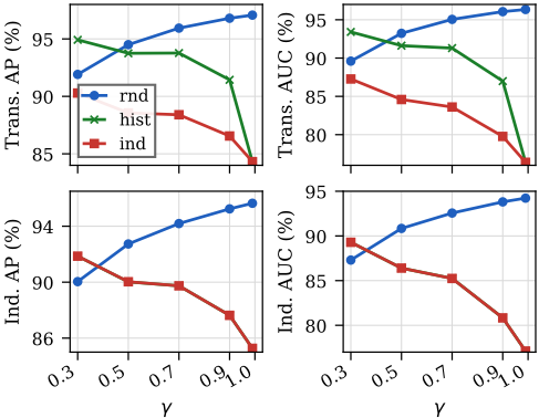
Hyperparameter Sensitivity. Figure 4 studies γ on UCI under random, historical, and inductive evaluation in both transductive and inductive settings.
The parameter γ controls the proportion of hard negatives during training. Lower γ improves hist and ind settings by exposing the model to harder negatives, but can slightly hurt rnd evaluation because excessive hard negatives are less useful for simpler random tests. Thus, γ should be calibrated to balance robustness and easy-case performance.
7 Conclusion
We introduced ATNSF, a temporal link prediction framework that combines hybrid negative sampling with a pairwise softmax objective. By injecting historical hard negatives during training and optimizing positive-negative rankings directly, ATNSF reduces the limitations of random negative sampling and pointwise losses. Experiments across transductive and inductive settings show that this design improves robustness to challenging negatives while maintaining efficient training. The results further suggest that negative sampling and loss design should be considered jointly: temporally plausible negatives make training signals more informative, and the pairwise objective helps the model exploit these signals without treating each negative independently. Future work can study adaptive schedules for the hard-negative ratio and extend the framework to richer temporal graph architectures.
Acknowledgments
We thank the anonymous reviewers for their constructive comments. Heng Zhang is partially supported by the National Science and Technology Major Project (2025ZD1606200), Youth Innovation Promotion Association CAS (2023120), and National Natural Science Foundation of China (62002350).
@inproceedings{ijcai2026p302,
  title     = {History Doesn’t Repeat, but Its Patterns Echo: A Parallel Pairwise Negative-Sampling Framework for Temporal Link Prediction},
  author    = {Jiang, Yongchun and Zhang, Heng and Gao, Jian and Zheng, Xin},
  booktitle = {Proceedings of the Thirty-Fifth International Joint Conference on
               Artificial Intelligence, {IJCAI-26}},
  publisher = {International Joint Conferences on Artificial Intelligence Organization},
  editor    = {Diego Calvanese},
  pages     = {2717--2725},
  year      = {2026},
  month     = {8},
  note      = {Main Track},
  doi       = {10.24963/ijcai.2026/302},
  url       = {https://doi.org/10.24963/ijcai.2026/302},
}
TY - CPAPER TI - History Doesn’t Repeat, but Its Patterns Echo: A Parallel Pairwise Negative-Sampling Framework for Temporal Link Prediction AU - Jiang, Yongchun AU - Zhang, Heng AU - Gao, Jian AU - Zheng, Xin T2 - Proceedings of the Thirty-Fifth International Joint Conference on Artificial Intelligence, IJCAI-26 PB - International Joint Conferences on Artificial Intelligence Organization PY - 2026 SP - 2717 EP - 2725 DO - 10.24963/ijcai.2026/302 UR - https://doi.org/10.24963/ijcai.2026/302 ER -Copied
Machine-readable versions of this paper, for tools and AI agents:





