
JointScaler: A Hierarchical Multi-Indicator Distribution Forecasting Approach for Uncertainty-Aware Joint Scaling in Cloud Services
Proceedings of the Thirty-Fifth International Joint Conference on Artificial Intelligence. Main Track. Pages 2906-2914.
https://doi.org/10.24963/ijcai.2026/323
Keywords
- Data Mining: Applications
- Data Mining: Mining spatial and/or temporal data
- Data Mining: Parallel, distributed and cloud-based high performance mining
Abstract
Proactive scaling improves cloud resource efficiency by forecasting system-relevant indicators and dynamically provisioning resources to maximize utilization while satisfying quality requirements. Existing approaches forecast service indicators in isolation, ignore forecasting uncertainty, and scale resource types independently, violating bundled resource constraints and degrading service quality. Therefore, we propose JointScaler, a learning-based framework for multi-indicator distribution forecasting and uncertainty-aware scaling. It captures inter-indicator dependencies via hierarchical attention, models dynamic uncertainties with normalizing flows, and leverages full predictive distributions to optimize bundled resource allocations under quality requirements. Evaluated on 4 real-world datasets, JointScaler improves point and distribution forecasting accuracy by 5.87% and 14.74%, outperforming 12 advanced baselines. In a week-long A/B test on a payment application’s cloud platform, it reduced GPU and CPU usage by 2,400+ and 37,000+ hours with stable service quality, delivering significant economic benefits.
- [Alibaba, 2018] Alibaba. Alibaba cluster trace v2018. https: //github.com/alibaba/clusterdata/tree/v2018, 2018. Link
- [Burns and Oppenheimer, 2016] Brendan Burns and David Oppenheimer. Design patterns for container-based dis- tributed systems. In USENIX Workshop on Hot Topics in Cloud Computing, 2016.
- [Cai et al., 2025] Zhicheng Cai, Hang Wu, Xu Jiang, Xiaop- ing Li, and Rajkumar Buyya. Deep learning and feed- back control based container auto-scaling for cloud native micro-services. IEEE Transactions on Service Computing (TSC), 18(5):2714-2725, 2025.
- [Chen et al., 2023a] Jiadong Chen, Yang Luo, Xiuqi Huang, Fuxin Jiang, Yangguang Shi, Tieying Zhang, and Xiaofeng Gao. IPOC: an adaptive interval prediction model based on online chasing and conformal inference for large-scale systems. In ACM SIGKDD Conference on Knowledge Dis- covery and Data Mining, pages 202-212, 2023.
- [Chen et al., 2023b] Si-An Chen, Chun-Liang Li, Nate Yo- der, Sercan Arik, and Tomas Pfister. Tsmixer: An all-mlp architecture for time series forecasting. Transcations on Machine Learning Research (TMLR), 2023.
- [Chen et al., 2026] Jiadong Chen, Yang Luo, Xiuqi Huang, Fuxin Jiang, Yangguang Shi, Tieying Zhang, and Xi- aofeng Gao. Uncertainty-aware online time series multi- step forecasting framework in cloud systems. IEEE Trans- actions on Knowledge and Data Engineering (TKDE), 38(5):3277-3290, 2026.
- [Fan et al., 2024] Xinyao Fan, Yueying Wu, Chang Xu, Yuhao Huang, Weiqing Liu, and Jiang Bian. MG-TSD: multi-granularity time series diffusion models with guided learning process. In International Conference on Learning Representations (ICLR), 2024.
- [Flunkert et al., 2017] Valentin Flunkert, David Salinas, and Jan Gasthaus. Deepar: Probabilistic forecasting with au- toregressive recurrent networks. CoRR, abs/1704.04110, 2017.
- [Gao et al., 2025] Mohan Gao, Kexin Xu, Xiaofeng Gao, Tengwei Cai, and Haoyuan Ge. Spatial-temporal heteroge- nous graph contrastive learning for microservice workload prediction. In Toby Walsh, Julie Shah, and Zico Kolter, ed- itors, Advancement of Artificial Intelligence (AAAI), pages 11681-11689, 2025.
- [Gao et al., 2026] Mohan Gao, Zhemeng Yu, Yang Luo, Lin- tao Ma, Yinbo Sun, Yuchen Fang, and Xiaofeng Gao. Macro-micro collaborative learning for logical data center microservice indicators forecasting. In ACM Web Confer- ence 2026 (WWW), pages 5010-5020, 2026.
- [Gneiting and Ranjan, 2011] Tilmann Gneiting and Roopesh Ranjan. Comparing density forecasts using threshold-and quantile-weighted scoring rules. Journal of Business & Economic Statistics, 29(3):411-422, 2011.
- [Granger, 1969] Clive WJ Granger. Investigating causal rela- tions by econometric models and cross-spectral methods. Econometrica: journal of the Econometric Society, pages 424-438, 1969.
- [Hang et al., 2024] Haitian Hang, Xiu Tang, Jianling Sun, Lingfeng Bao, David Lo, and Haoye Wang. Robust auto- scaling with probabilistic workload forecasting for cloud databases. In IEEE International Conference on Data En- gineering, (ICDE), pages 4016-4029, 2024.
- [Hu et al., 2025] Yifan Hu, Guibin Zhang, Peiyuan Liu, Disen Lan, Naiqi Li, Dawei Cheng, Tao Dai, Shu-Tao Xia, and Shirui Pan. Timefilter: Patch-specific spatial-temporal graph filtration for time series forecasting. In International Conference on Machine Learning (ICML), 2025.
- [Hua et al., 2023] Qin Hua, Dingyu Yang, Shiyou Qian, Hanwen Hu, Jian Cao, and Guangtao Xue. Kae-informer: A knowledge auto-embedding informer for forecasting long-term workloads of microservices. In ACM The Web Conference (WWW), pages 1551-1561, 2023.
- [Liu et al., 2022] Shizhan Liu, Hang Yu, Cong Liao, Jian- guo Li, Weiyao Lin, Alex X. Liu, and Schahram Dust- dar. Pyraformer: Low-complexity pyramidal attention for long-range time series modeling and forecasting. In Inter- national Conference on Learning Representations (ICLR), 2022.
- [Liu et al., 2024] Yong Liu, Tengge Hu, Haoran Zhang, Haixu Wu, Shiyu Wang, Lintao Ma, and Mingsheng Long. itransformer: Inverted transformers are effective for time series forecasting. In International Conference on Learn- ing Representations (ICLR), 2024.
- [Liu, 2018] Chris Liu. Fisher-model: Use bi-lstm to pre- dict load in container. https://github.com/chrisliu1995/ Fisher-model, 2018. Link
- [Luo et al., 2024a] Yang Luo, Mohan Gao, Zhemeng Yu, Haoyuan Ge, Xiaofeng Gao, Tengwei Cai, and Guihai Chen. Integrating system state into spatio temporal graph neural network for microservice workload prediction. In ACM SIGKDD Conference on Knowledge Discovery and Data Mining, 2024.
- [Luo et al., 2024b] Yang Luo, Shiyu Wang, Zhemeng Yu, Wei Lu, Xiaofeng Gao, Lintao Ma, and Guihai Chen. Adaptive two-stage cloud resource scaling via hierarchical multi-indicator forecasting and bayesian decision-making. CoRR, abs/2408.01000, 2024.
- [Luo et al., 2026] Yang Luo, Yiheng Wang, Lingyi Long, Tengwei Cai, Xiaofeng Gao, and Guihai Chen. Stdps: State-aware spatio-temporal workload distribution predic- tion for cloud service scaling. IEEE Transactions on Ser- vices Computing (TSC), 2026. [Meta, 2024] Meta. Building meta's genai infrastructure. https://engineering.fb. com/2024/03/12/data-center-engineering/ building-metas-genai-infrastructure/, 2024. Link
- [Murad et al., 2025] Md Mahmuddun Nabi Murad, Mehmet Aktukmak, and Yasin Yilmaz. Wpmixer: Efficient multi- resolution mixing for long-term time series forecasting. In Advancement of Artificial Intelligence (AAAI), pages 19581-19588, 2025.
- [Nie et al., 2023] Yuqi Nie, Nam H. Nguyen, Phanwadee Sinthong, and Jayant Kalagnanam. A time series is worth 64 words: Long-term forecasting with transformers. In International Conference on Learning Representations (ICLR), 2023. [OpenAI, 2021] OpenAI. Scaling kubernetes to 7,500 nodes. https://openai.com/research/ scaling-kubernetes-to-7500-nodes, 2021. Link
- [Pan et al., 2023] Zhicheng Pan, Yihang Wang, Yingying Zhang, Sean Bin Yang, Yunyao Cheng, Peng Chen, Chen- juan Guo, Qingsong Wen, Xiduo Tian, Yunliang Dou, Zhiqiang Zhou, Chengcheng Yang, Aoying Zhou, and Bin Yang. Magicscaler: Uncertainty-aware, predictive au- toscaling. Proceedings of the VLDB Endowment (VLDB), 16(12):3808-3821, 2023.
- [Qiu et al., 2020] Haoran Qiu, Subho S. Banerjee, Saurabh Jha, Zbigniew T. Kalbarczyk, and Ravishankar K. Iyer. FIRM: an intelligent fine-grained resource management framework for slo-oriented microservices. In USENIX Symposium on Operating Systems Design and Implemen- tation, OSDI, pages 805-825, 2020.
- [Rebjock et al., 2020] Quentin Rebjock, Valentin Flunkert, Tim Januschowski, Laurent Callot, and Joel Castellon. A simple and effective predictive resource scaling heuristic for large-scale cloud applications. In International Work- shop on Applied AI for Database Systems and Applica- tions, Held with VLDB, 2020.
- [Rzadca et al., 2020] Krzysztof Rzadca, Pawel Findeisen, Jacek Swiderski, Przemyslaw Zych, Przemyslaw Broniek, Jarek Kusmierek, Pawel Nowak, Beata Strack, Piotr Witu- sowski, Steven Hand, and John Wilkes. Autopilot: work- load autoscaling at google. In ACM EuroSys Conference, pages 16:1-16:16, 2020.
- [Tashiro et al., 2021] Yusuke Tashiro, Jiaming Song, Yang Song, and Stefano Ermon. CSDI: conditional score-based diffusion models for probabilistic time series imputation. In Advances in Neural Information Processing Systems (NeurIPS), pages 24804-24816, 2021.
- [Verma et al., 2015] Abhishek Verma, Luis Pedrosa, Mad- hukar Korupolu, David Oppenheimer, Eric Tune, and John Wilkes. Large-scale cluster management at google with borg. In European Conference on Computer Systems (Eu- roSys). ACM, 2015.
- [Wang et al., 2023] Shiyu Wang, Yinbo Sun, Xiaoming Shi, Shiyi Zhu, Lintao Ma, James Zhang, Yangfei Zheng, and Liu Jian. Full scaling automation for sustainable develop- ment of green data centers. In International Joint Confer- ence on Artificial Intelligence, (IJCAI), pages 6264-6271, 2023. IJCAI
- [Wang, 2024] Shiyu Wang. Neuralreconciler for hierarchical time series forecasting. In ACM International Conference on Web Search and Data Mining (WSDM), pages 731-739, 2024.
- [Zeng et al., 2023] Ailing Zeng, Muxi Chen, Lei Zhang, and Qiang Xu. Are transformers effective for time series fore- casting? In Conference on Artificial Intelligence (AAAI), pages 11121-11128, 2023.
- [Zhang and Yan, 2023] Yunhao Zhang and Junchi Yan. Crossformer: Transformer utilizing cross-dimension de- pendency for multivariate time series forecasting. In Inter- national Conference on Learning Representations (ICLR), 2023.
- [Zou et al., 2024] Aaron Zou, Wei Lu, Zhibo Zhu, Xingyu Lu, Jun Zhou, Xiaojin Wang, Kangyu Liu, Kefan Wang, Renen Sun, and Haiqing Wang. Optscaler: A collabora- tive framework for robust autoscaling in the cloud. Pro- ceedings of the VLDB Endowment (VLDB), 17(12):4090- 4103, 2024.
References were extracted automatically from the PDF and may contain errors.
Full text extracted automatically from the PDF; figures, tables and equations may differ. The PDF is the version of record.
1 Introduction
The rising demand for computing power drives major investments in cloud infrastructure. For instance, Meta uses more than 24,000 NVIDIA H100 GPUs, and OpenAI runs over 7,500 GPU servers [Meta, 2024; OpenAI, 2021]. In large-scale cloud systems, services must meet performance requirements defined in Service Level Agreements (SLAs), such as maximum acceptable response time. To avoid breaching SLAs, providers often a/ llocate more resources than needed, leading to consistently low utilization and significant economic waste [Wang et al., 2023; Luo et al., 2024a]. To balance cost and reliability, many cloud platforms now use proactive scaling [Zou et al., 2024; Luo et al., 2024b;
∗Xiaofeng Gao is the Corresponding Author
1 Code: https://github.com/Floating-LY/Joint-Scaler
Luo et al., 2026]. This method predicts key service indicators and adjusts resource allocation in advance to maintain SLA compliance while improving efficiency.
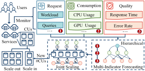
The upper part of Fig.1 shows the typical resource scaling process. The lower part illustrates our proactive scaling framework, consisting of two stages: forecasting and scaling.
In the forecasting stage, the service monitors multiple indicator series that together describe its operational state. Although these indicators are observed separately, we find that they naturally cluster into different functional levels that reflect how the service works: (1) Request-Level captures incoming user demand; (2) Consumption-Level measures internal resource usage needed; and (3) Quality-Level reflects the service performance. This hierarchical structure implies a directional dependence: request dynamics drive resource consumption, which in turn determines the quality of service.
In the scaling stage, the system allocates resources in atomic Computational Units (CUs). Instead of assigning individual CPU cores or GPUs independently, cloud systems bundle heterogeneous resources such as 4 CPU cores and 1 GPU card into a fixed CU. This reduces fragmentation and simplifies scheduling in distributed environments [Verma et al., 2015]. As a result, scaling decisions must respect joint constraints across different resource types within each CU.
Despite these insights, current scaling methods face serious challenges, as we observed when operating a cloud platform for a payment application with over one billion global users.
Challenge 1: Modeling Hierarchical Multi-Indicators. Existing cloud forecasters treat indicators as isolated signals [Wang et al., 2023; Luo et al., 2024a; Gao et al., 2025; Chen et al., 2026], ignoring their functional hierarchy and dependence ordering confirmed via Granger analysis in Sec. 2.1. Without modeling this hierarchy, temporal patterns cannot propagate correctly across levels, reducing forecast accuracy.
Challenge 2: Estimating Forecasting Uncertainty. User request patterns are inherently variable, causing dynamic uncertainty in service indicators. Yet most approaches rely on single-point predictions [Chen et al., 2023a; Gao et al., 2026], fail to account for potential SLA violations. Recent methods explore probabilistic forecasts but assume fixed Gaussian distributions [Zou et al., 2024], which cannot capture the dynamic forecasting uncertainty observed in Sec. 2.2.
Challenge 3: Scaling Bundled Resources. Current scalers [Zou et al., 2024; Hang et al., 2024; Cai et al., 2025] often optimize CPU, GPU, and other resources separately. This ignores both the atomic nature of CUs and the bundled coupling between resource types. Their scaling result is often either violating quality requirements or leading to redundant resources violating SLA as demonstrated in Sec. 2.3.
To tackle these challenges, we propose JointScaler, a new proactive scaling framework that integrates two key parts. The Multi-Indicator Distribution Forecaster clusters service indicators into hierarchical levels to reflect their semantic roles in system dynamics. We propose the hierarchical attention to model directional inter-indicator dependencies (Challenge 1), and leverage Normalizing Flows (NFs) to capture flexible forecast uncertainties (Challenge 2). The Uncertainty-Aware Joint Distribution-Aware Scaler includes a Resource Allocation Judger that jointly reasons over multi-indicator uncertainty distributions for bundled Computational Units, and an SLA-Aware Weight Adapter that dynamically adjusts scaling algorithms based on real-time SLA violation risk quantification to preserve service quality (Challenge 3). To the best of our knowledge, JointScaler is the first scaling framework that explicitly encodes hierarchical dependencies among cloud service indicators. It jointly forecasts their full distributions and performs uncertainty-aware scaling under resource bundling constraints. In summary, we:
- Identify a new AI research problem: forecasting hierarchical multi-indicators in cloud services, bridging timeseries modeling and practical resource management.
- Propose JointScaler, a novel AI framework for cloud service scaling, combining multi-indicator distributional forecasting with joint scaling under bundled resources.
- Achieve state-of-the-art performance on four heterogeneous datasets, outperforming 12 baselines and saving 2,400 GPU-hours and 37,000 CPU-hours in scaling test while maintaining 98.45% SLA compliance.
2 Data Analysis and Observation
To understand the challenges of proactive scaling in cloud services, we analyze service indicators from two real-world sources: the public Fisher dataset [Liu, 2018] and GPU traces collected over one week from a large-scale payment platform.
2.1 Hierarchical Dependencies
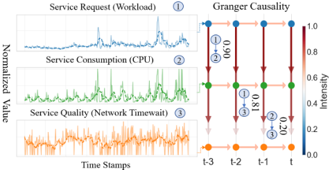
To evaluate the hierarchical structure of service indicators, we apply the same level clustering to the Fisher dataset and show the result for a representative service in Fig.2. Granger causality analysis [Granger, 1969] illustrates significant directional dependence between the levels, supporting our observed hierarchical dependencies. Modeling these multiindicator dependencies can enhance forecasting accuracy.
2.2 Forecasting Uncertainty
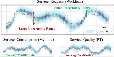
To investigate forecasting uncertainty, we present multiindicator distribution forecasts of JointScaler for a model inference service in the payment platform over 24 hours, as shown in Fig. 3. We observe that: (1) for the same indicator, the uncertainty intervals vary significantly across time; and (2) different indicators exhibit distinct levels of forecasting uncertainty. Point forecasts fall short in capturing these temporal and cross-indicator uncertainties, limiting the accuracy of scaling decisions. Distributional forecasting is thus essential for reliable cloud service resource management.
2.3 Joint Scaling Heterogeneous Resources
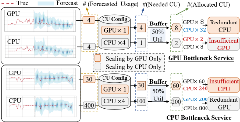
Cloud services consume heterogeneous resources with varying consumption patterns. Fig.4 illustrates two real-world services from a payment platform: one GPU-dominant and one CPU-dominant. Relying on a single resource for scaling leads to severe imbalances. For instance, in a GPU-dominant service, scaling based only on GPU demand results in redundant CPUs; yet scaling based solely on CPU usage leaves GPUs severely insufficient, degrading service quality. Similar imbalances occur for CPU-dominant services. This imbalance underscores a key insight: effective scaling in heterogeneous environments must jointly consider multiple resource types to balance efficient resource utilization and service quality.
3 ProblemDefinition
We begin by the basic concepts of proactive scaling first.
Definition 1 (Indicator Series). Indicator series represent the status of a service at different time stamps, including information on service requests, consumption ,and quality . The indicator series are denoted as X ∈ RN×T , where N and T denote the number of indicators and time stamps, respectively. In addition, We use Xr ∈ RR×T , Xc ∈ RC×T , and Xq ∈ RQ×T denotes the service requests, consumption, quality indicators where R + C + Q = N .
Definition 2 (Level Identification). Level Identification is denoted by an array L ∈ ZN , where each element Ln ∈ {1, . . . ,Lmax} represents the semantic level of the corresponding indicator Xn in the hierarchical structure.
Based on indicator series and level identification, we aim to predict future distributions of these indicators.
Task 1 (Forecasting). Given indicator series X ∈ RN×T and level information L ∈ ZN , We forecast the distribution of the indicators at time stamp T + 1. We denote the forecast distribution as D ∈ RN×S , where S is the number of possible states in the distribution of each indicator.
Then we define the atomic computational unit for scaling in cloud services, which may be referred to by different names depending on the cloud architecture, such as containers in distributed systems [Burns and Oppenheimer, 2016].
Definition 3 (Computational Unit). ACU comprises a combination of compute resources such as CPU, GPU, and Memory. The CUs have a specific configuration denoted as O ∈
ZC , where each element Oc represents the quantity of the c-th resource type. Here C corresponds to the number of service consumption indicators. All computational units for a cloud service share identical configurations.
We finally determine the optimal number of CUs required based on the distributions of indicators and the CU configuration, ensuring the service quality indicators meet SLAs.
Task 2 (Scaling). Given the predicted distributions D and CU configuration O, the goal of the scaling algorithm A is to determine the appropriate number of CUs U to allocate. The optimal number is denoted by Uopt = A(D,O), ensuring service quality indicators meet the specified SLAs.
4 Forecasting Future Distributions
JointScaler predicts service indicator distributions via two core components: hierarchical relationship modeling and distribution transformation. Input indicator series are encoded into embeddings to capture temporal patterns, with hierarchical attention modeling inter-indicator dependencies. The resulting representation is projected into an initial Gaussian distribution, then transformed via Normalizing Flows to generate flexible distributions that better capture service variability and uncertainty. Fig. 5 presents JointScaler's framework.
4.1 Capturing Hierarchical Dependencies
This section addresses Challenge 1 by extracting temporal patterns and hierarchical dependencies from indicator series using Indicator Embedding and Hierarchical Attention.
Indicator Embedding
JointScaler begins with indicator series X ∈ RN×T , where N is the number of service indicators and T denotes the sequence length. Following recent findings in multivariate time series modeling [Liu et al., 2024], we embed along the variable dimension N rather than the temporal axis T , as it better captures inter-indicator correlations in cloud services.
To enrich temporal patterns, we extract F periodic and time features (e.g. day-of-week) as Tf ∈ RF×T and concatenate them with X to form an augmented input ˜X = [X; Tf ] ∈ R(N+F )×T . This matrix is projected into a shared embedding space via a learnable linear transformation:
where We ∈ RD×(N+F) and be ∈ RD are trainable parameters, and D is the embedding dimension. The resulting E serves as the initial representation for hierarchical attention.
Hierarchical Attention
We propose a Dependency-Constrained Hierarchical Attention mechanism to explicitly model the directional dependency structure among service indicators, addressing the disordered multi-indicator relationship described in Challenge 1. Each indicator is assigned a semantic level ln ∈ {1, 2, ...,Lmax}, where lower levels (e.g., l = 1) correspond to foundational signals like request load and higher levels represent derived states such as service latency and SLA compliance.
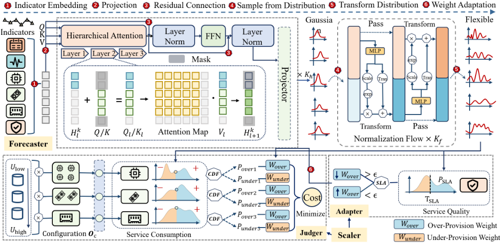
To enforce strict bottom-up information flow, we partition all N + F tokens into disjoint level-specific groups. Let ˜L ∈ {1, . . . ,Lmax}N+F be the extended level assignment. For each level l ∈ {1, . . . ,Lmax}, define the index set Gl = {i ∈ {1, . . . ,N + F} | ˜li = l}. The collection {Gl}Lmax l=1 forms a partition satisfing: Gi ∩ Gj = ∅ for all i ̸= j, ⋃Lmax l=1 Gl = {1, . . . ,N +F}.
In each block, we first compute shared linear projections for query, key, and value as denoted in Eqn. (2).
where WQ,WK,WV ∈ RD×D . We then process levels sequentially. Let Hk1 =Hk be the initial token state.
For level l, we define the attention context as the union of current and previous level tokens to enable cross-level interaction while preserving hierarchical directionality in Eqn. (3):
Query, key, and value vectors are drawn from the current state restricted to Cl in Eqn. (4). Hkl [Cl, :] denotes the submatrix of Hk formed by selecting all rows indexed by the set Cl.
This extraction step ensures that subsequent attention computation is confined to the functional scope of level l. We then conduct attention operation over Cl as in Eqn. (5) and extract only the output for tokens in Gl as Eqn. (6) denotes:
The residual state is then updated exclusively at Gl, leaving all other tokens unchanged as in Eqn. (7):
This design enforces bottom-up dependence by allowing each level to attend to the latest representations of its direct dependencies. Its worst-case time complexity is O((N + F)2D), matching that of standard self-attention. In typical hierarchical settings with multiple levels L, attention is restricted to small, level-specific contexts, leading to lower computational cost in practice.
The outputs from all layers are summed, normalized, and refined by a feed-forward network as in Eqn. (8).
where FFN(·) = Dropout(ReLU(·W1 + b1)W2 + b2).
After Kh blocks the embeddings for the N service indicators are extracted as HKh :N ∈ RN×D . These are mapped to the parameters of a Gaussian distribution as in Eqn. (9).
4.2 Transforming Gaussian Distributions
To capture dynamic uncertainties in real workloads, we transform the base Gaussian into a flexible distribution by Normalizing Flows [Wang, 2024]. It addresses Challenge 2 by enabling density estimation beyond parametric assumptions.
Starting from D(G) = z(0) ∼ N(µ, diag(σ2 )), we apply Kf invertible layers. At layer k, z(k) is split into two halves. The first half generates scale and translation parameters in Eqn. (10). s adjusts local variance to capture tail behavior, t enables asymmetric shifts to model skewed indicators.
The second half is then transformed as in Eqn. (11):
The roles are swapped to update the first half, and the full output is reconstructed as in Eqn. (12):
Each coupling transformation is invertible and allows exact computation of the output probability density from the base Gaussian. It enables likelihood evaluation as in Eqn. (13):
This flow-based design adapts to the true empirical shape of each indicator's dynamic uncertainty. As a result, JointScaler supports both point forecasting and distributional quantification, essential for robust scaling decisions under uncertainty.
5 Scaling under Uncertainty
As highlighted in Challenge 3, scaling based on point predictions ignores inherent uncertainty. Therefore, we propose the Uncertainty-aware Joint Distribution-Aware Scaler, utilizing full forecast distributions to compute expected costs for each candidate number of CUs to allocate, balancing resource efficiency and quality requirements in resource allocation.
The proposed scaler consists of two main components: an SLA-Aware Weight Adapter and a Resource Allocation Judger. The scaling algorithm A takes the following inputs:
- D ∈ RN×S : forecast demand distribution
- O ∈ RC : Configurations for computational units
- [Ulow,Uhigh]: Operational range for CU count
- Wover,Wunder: Penalty weights
- TSLA: SLA threshold for service quality
SLA-Aware Weight Adapter. It adjusts penalty weights Wover and Wunder to balance SLA compliance and resource efficiency. The SLA violation probability is as Eqn. (14):
where Dp represents the distribution of service quality indicators (e.g., latency) and TSLA denotes the SLA threshold. When PSLA exceeds a predefined risk threshold ϵ, the over-provisioning penalty is reduced via Wover ← α · Wover (α ∈ (0, 1)) to prioritize resource allocation. Conversely, Wover is scaled up using β · Wover (β > 1) when SLA risks are low, penalizing excessive resource consumption.
Resource Allocation Judger. The second component determines the optimal number of CUs within the operational
- range [Ulow,Uhigh] by calculating the cost associated with over provisioning and under provisioning risks through:
- Resource Allocation: Calculate the potential resources to be allocated as U ×Oc, where U is the number of CUs and Oc represents the configuration of each CU.
- Provisioning Probabilities: Estimate both overprovisioning probability P over and under-provisioning probability Punder as follows: Pover[c] = P(Dc > U ×Oc), P under [c] = P (Dc < U ×Oc), The cumulative distribution function (CDF) is used to evaluate these probabilities, which can be estimated either through kernel density estimation or by calculating sample proportions fromDc.
- Cost Estimation: Compute the cost for U by Eqn. (15). Here, Wover ∈ RC and Wunder ∈ RC are weights for over and under provisioning risks, respectively.
Finally, the CU count that minimizes the expected cost is selected as the optimal value Uopt. The scaler runs continuously in each decision cycle, dynamically adjusting penalty weights via an SLA-aware adapter based on service risks.
6 Experiments
In this section, we conduct a series of experiments to evaluate JointScaler 's forecasting and scaling performance.
Datasets
We employ 4 real-world cloud traces across various architectures to test JointScaler's robust performance: (1) Pay GPU: From a large payment platform, covering 100 high-load GPU inference services over a week (3441 GPUs), representing high-performance GPU environments. (2) Pay CPU: From the same platform, including 100 CPU services over a week (120,248 CPU cores), representing CPU-intensive infrastructure. (3) Ali [Alibaba, 2018] : From Alibaba Cluster Trace, recording indicators from 50 machines over 8 days, reflecting typical machine-based architectures. (4) Fisher [Liu, 2018]: Workload trace from 10 Kubernetes containers over 30 days, representing containerized environments.
Data preprocessing
We use MinMax normalization to standardize all indicators and aggregate indicators into 10-minute intervals using the maximum value for each interval. This aggregation alleviates SLA violations due to under-provisioning. We divide datasets into training, validation, and testing sets in a 7:1:2 ratio for robust model evaluation. Following Def. 1, we categorized service indicators into levels such as request, consumption, and quality, generating Level Identification as the input.
Baselines
For the forecasting task, we compare with 12 advanced baselines containing probabilistic prediction methods: DeepAR [Flunkert et al., 2017], CSDI [Tashiro et al., 2021], MGTSD [Fan et al., 2024], and multivarate prediction methods: Pyraformer [Liu et al., 2022], DLinear [Zeng et al., 2023], PatchTST [Nie et al., 2023], Crossformer [Zhang and Yan, 2023], TSMixer [Chen et al., 2023b], iTransformer [Liu et al., 2024], TimeFilter [Hu et al., 2025], WPMixer [Murad et al., 2025], KAEInformer [Hua et al., 2023].
| Datasets | Pay GPU | Pay CPU | Ali | Fisher | Avg. Rank | |||||||||
|---|---|---|---|---|---|---|---|---|---|---|---|---|---|---|
| T | 72 | 144 | 288 | 72 | 144 | 288 | 72 | 144 | 288 | 72 | 144 | 288 | ||
| DeepAR | MSE | 0.0225 | 0.0291 | 0.0366 | 0.3593 | 0.4260 | 0.4997 | 0.0044 | 0.0054 | 0.0066 | 0.0695 | 0.0604 | 0.0562 | 7.0417 |
| CSDI | MSE | 0.0374 | 0.0409 | 0.0513 | 0.2674 | 0.2680 | 0.2998 | 0.0172 | 0.0116 | 0.0134 | 0.0766 | 0.0968 | 0.0934 | 8.9167 |
| MG-TSD | MSE | 0.0331 | 0.0357 | 0.0443 | 0.1258 | 0.1718 | 0.2196 | 0.0318 | 0.0323 | 0.0349 | 0.0650 | 0.0663 | 0.0757 | 7.7500 |
| Pyraformer | MSE | 0.0227 | 0.0241 | 0.0374 | 0.0676 | 0.1084 | 0.1441 | 0.0042 | 0.0056 | 0.0062 | 0.0461 | 0.0469 | 0.0483 | 3.5833 |
| DLinear | MSE | 0.0350 | 0.0419 | 0.0413 | 0.1365 | 0.1748 | 0.2442 | 0.0112 | 0.0145 | 0.0167 | 0.0500 | 0.0574 | 0.0557 | 7.0000 |
| PatchTST | MSE | 0.0202 | 0.0267 | 0.0481 | 0.0327 | 0.0604 | 0.1219 | 0.0044 | 0.0049 | 0.0058 | 0.0467 | 0.0472 | 0.0485 | 3.5000 |
| Crossformer | MSE | 0.8261 | 1.2853 | 1.6736 | 0.3639 | 0.4071 | 0.5541 | 0.0891 | 0.0962 | 0.0612 | 0.0587 | 0.0616 | 0.0640 | 11.1667 |
| TSMixer | MSE | 0.2013 | 0.0880 | 0.5510 | 0.2997 | 0.2465 | 0.1610 | 0.0410 | 0.0246 | 0.0239 | 0.0581 | 0.0863 | 0.1046 | 9.5000 |
| iTransformer | MSE | 0.0179 | 0.0248 | 0.0476 | 0.0337 | 0.0683 | 0.1103 | 0.0047 | 0.0055 | 0.0071 | 0.0470 | 0.0489 | 0.0496 | 4.4167 |
| TimeFilter | MSE | 0.2602 | 0.2812 | 0.7984 | 0.2860 | 0.3579 | 0.3694 | 0.1224 | 0.1288 | 0.1239 | 0.0921 | 0.0918 | 0.1016 | 11.5833 |
| WPMixer | MSE | 0.0322 | 0.0385 | 0.0463 | 0.0786 | 0.0961 | 0.0834 | 0.0035 | 0.0041 | 0.0067 | 0.0467 | 0.0475 | 0.0477 | 3.8750 |
| KAEInformer | MSE | 0.0992 | 0.1198 | 0.4716 | 0.2723 | 0.2921 | 0.3266 | 0.1202 | 0.1384 | 0.1308 | 0.1485 | 0.1565 | 0.1639 | 11.4167 |
| JointScaler | MSE | 0.0171 | 0.0229 | 0.0355 | 0.0323 | 0.0448 | 0.0762 | 0.0039 | 0.0048 | 0.0061 | 0.0453 | 0.0458 | 0.0474 | 1.3333 |
| DeepAR | CRPS | 0.0706 | 0.0807 | 0.0992 | 0.2142 | 0.2170 | 0.2351 | 0.0399 | 0.0492 | 0.0542 | 0.1481 | 0.1390 | 0.1276 | 5.2500 |
| CSDI | CRPS | 0.1214 | 0.1302 | 0.1828 | 0.5457 | 0.5273 | 0.5369 | 0.0730 | 0.0588 | 0.0613 | 0.1634 | 0.2282 | 0.1481 | 9.4167 |
| MG-TSD | CRPS | 0.1454 | 0.2628 | 0.3062 | 0.3317 | 0.4722 | 0.5837 | 0.0535 | 0.0729 | 0.0852 | 0.1840 | 0.1991 | 0.2057 | 10.2500 |
| Pyraformer | CRPS | 0.0781 | 0.0859 | 0.1140 | 0.0891 | 0.1146 | 0.1519 | 0.0327 | 0.0401 | 0.0473 | 0.1141 | 0.1172 | 0.1283 | 3.9167 |
| DLinear | CRPS | 0.1176 | 0.1372 | 0.1323 | 0.1920 | 0.2066 | 0.2356 | 0.0821 | 0.0855 | 0.0888 | 0.1448 | 0.1606 | 0.1450 | 7.3333 |
| PatchTST | CRPS | 0.0719 | 0.0893 | 0.1363 | 0.0708 | 0.0921 | 0.1298 | 0.0328 | 0.0351 | 0.0426 | 0.1143 | 0.1159 | 0.1195 | 3.1667 |
| Crossformer | CRPS | 0.6652 | 0.9662 | 1.1406 | 0.3067 | 0.3866 | 0.4622 | 0.2359 | 0.2496 | 0.2048 | 0.1545 | 0.1596 | 0.1594 | 10.8333 |
| TSMixer | CRPS | 0.3686 | 0.2160 | 0.5487 | 0.2347 | 0.2449 | 0.2060 | 0.1550 | 0.1235 | 0.1166 | 0.1484 | 0.1691 | 0.1963 | 9.1667 |
| iTransformer | CRPS | 0.0708 | 0.0892 | 0.1328 | 0.0711 | 0.0962 | 0.1295 | 0.0340 | 0.0390 | 0.0482 | 0.1160 | 0.1200 | 0.1237 | 4.0417 |
| TimeFilter | CRPS | 0.4467 | 0.4358 | 0.7787 | 0.2958 | 0.3195 | 0.3170 | 0.2989 | 0.3145 | 0.3015 | 0.2008 | 0.1981 | 0.2037 | 11.4167 |
| WPMixer | CRPS | 0.0956 | 0.1095 | 0.1237 | 0.0710 | 0.1051 | 0.1089 | 0.0331 | 0.0390 | 0.0532 | 0.1165 | 0.1184 | 0.1199 | 4.1250 |
| KAEInformer | CRPS | 0.2333 | 0.2521 | 0.4958 | 0.2557 | 0.2875 | 0.3365 | 0.2798 | 0.3061 | 0.2957 | 0.2493 | 0.2573 | 0.2619 | 11.0833 |
| JointScaler | CRPS | 0.0563 | 0.0664 | 0.0890 | 0.0572 | 0.0730 | 0.0943 | 0.0289 | 0.0290 | 0.0399 | 0.0995 | 0.0940 | 0.1097 | 1.0000 |
Evaluation Metrics
We employ Mean Squared Error (MSE) to evaluate point prediction and Continuous Ranked Probability Score (CRPS) [Gneiting and Ranjan, 2011] for probabilistic forecasts. For probabilistic methods, we compute MSE from sampled forecasts; for point-based methods, we treat repeated point predictions as degenerate distributions to calculate CRPS. Lower RMSE and CRPS indicate better performance. This dualmetric evaluation comprehensively assesses model effectiveness in both point and distributional forecasting.
Parameter Settings
JointScaler is trained on an NVIDIA P100 GPU. The learning rate is set to 0.001, the batch size is set to 128, and the representation dimension d is set to 512. The numbers of Hierarchical Attention block and Normalizing Flow are both set to 2. All models are trained for 20 epochs, and the bestperforming model on the validation set is utilized for testing.
6.1 Forecasting Performance
Table 1 presents the results between JointScaler and baselines. The experimental data lead to several conclusions:
- JointScaler outperforms baselines in both point and probabilistic prediction across four service datasets, with average reduction of 5.87% in MSE and 14.74% in CRPS.
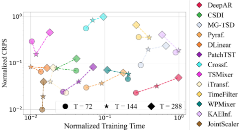
- JointScaler achieves high prediction accuracy while maintaining efficiency as illustrated in Fig. 7. Comparing to MLP-based methods such as TSMixer and DLinear that prioritize efficiency over accuracy, JointScaler 's indicator embed-
- ding makes its runtime relatively insensitive to input length T , enabling adaptability to varied input sizes.
- A counterintuitive trend emerges: larger input length T does not consistently improve prediction accuracy for realtime cloud services. It indicates longer series include obsolete historical patterns due to service adjustments or evolving conditions, introducing noise that degrades accuracy.
6.2 Ablation Study
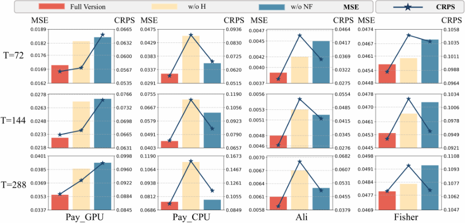
We conducted ablation studies to analyze the impact of key components. The outcomes are shown in Fig. 6.
- Replacing Hierarchical Attention with Full Attention (denoted "w/o H")-which computes pairwise attention coefficients for all indicators-worsens MSE and CRPS across all input lengths and datasets. For CPU services with stable indicator relationships, removing Hierarchical Attention increases MSE by 49.7% on average. It indicates Full Attention fails to account for hierarchical indicator relationships, confusing cross-layer information propagation. Thus, Hierarchical Attention is more effective for structured services.
- Impact of Normalizing Flow: Comparing with a variant using linear layers for Gaussian mapping ("w/o NF") shows significant increases in MSE and CRPS. It confirms NFs better capture indicator distributions, with larger gains in complex environments (Pay GPU, Ali, Fisher) due to its adaptability to intricate patterns. Thus, NF enhances performance in dynamic services, critical for accurate prediction.
6.3 Scaling Performance
We conduct a week-long A/B test on 10 large-scale GPU services in the payment application's cloud platform to evaluate our scaling performance. Key metrics include CPU/GPU usage hours (C Usage, G Usage), CPU/GPU utilization (C Uti, G Uti), and SLA compliance rate (SLAR). Lower resource usage with high SLAR indicates better performance.
We include 8 baselines. (1) Non-Proactive Methods: Rule-Based and Autopilot [Rzadca et al., 2020]; (2) Deterministic Proactive Methods: FIRM [Qiu et al., 2020], FSA [Wang et al., 2023]. (3) Probability Proactive Methods: FS [Rebjock et al., 2020], MagicScaler [Pan et al., 2023], Robust [Hang et al., 2024].
Table 2 confirms JointScaler's superiority, achieving higher resource utilization with 98.45% SLAR. Minor avoidable SLAR violations occur during occasional service restarts. Notably, JointScaler saved 37,000+ CPU core hours and 2,400+ GPU hours in a week without compromising service quality, translating to an estimated annual cost reduction of over $460,000 for the evaluated services. Greater gains are achievable across a broader range of services.
| Methods | C Usage | G Usage | C Uti | G Uti | SLAR |
|---|---|---|---|---|---|
| NoScale | 9.52e+5 | 4.50e+4 | 11.34% | 26.22% | 99.82% |
| Rule-Based | 2.78e+5 | 1.49e+4 | 26.75% | 45.28% | 98.74% |
| Autopilot | 2.92e+5 | 1.54e+4 | 26.89% | 44.65% | 91.04% |
| FIRM | 2.99e+5 | 1.61e+4 | 27.21% | 41.06% | 93.87% |
| FSA | 3.11e+5 | 1.61e+4 | 25.91% | 41.99% | 92.25% |
| Robust | 2.93e+5 | 1.59e+4 | 23.81% | 38.46 % | 98.78% |
| FS | 2.80e+5 | 1.50e+4 | 26.33% | 45.93% | 97.16% |
| MagicScaler | 2.79e+5 | 1.49e+4 | 26.65% | 46.68% | 95.91% |
| JointScaler | 2.41e+5 | 1.25e+4 | 33.65% | 55.37% | 98.45% |
7 Conclusion
We propose JointScaler, a proactive scaling framework that tackles a key AI challenge in cloud data centers: modeling hierarchical dependencies among multi-level service indicators. Unlike prior works that treat indicators independently and assume simple uncertainty distributions, JointScaler jointly captures nonlinear inter-indicator dynamics, uses normalizing flows for flexible forecast distributions, and enforces bundled CU constraints through an uncertainty-aware decision mechanism. It achieves higher forecasting accuracy and improves resource efficiency.
Acknowledgments
This work was supported by the National Key R&D Program of China [2024YFF0617700], the National Natural Science Foundation of China [U23A20309, 62172276, 62372296, 62272302], Shanghai Municipal Science and Technology Major Project [2021SHZDZX0102], and CCF-Ant Research Fund [CCF-AFSG RF20230408].
@inproceedings{ijcai2026p323,
  title     = {JointScaler: A Hierarchical Multi-Indicator Distribution Forecasting Approach for Uncertainty-Aware Joint Scaling in Cloud Services},
  author    = {Luo, Yang and Yu, Zhemeng and Fu, Yikang and LU, Wei and Ma, Lintao and Gao, Xiaofeng and Chen, Guihai},
  booktitle = {Proceedings of the Thirty-Fifth International Joint Conference on
               Artificial Intelligence, {IJCAI-26}},
  publisher = {International Joint Conferences on Artificial Intelligence Organization},
  editor    = {Diego Calvanese},
  pages     = {2906--2914},
  year      = {2026},
  month     = {8},
  note      = {Main Track},
  doi       = {10.24963/ijcai.2026/323},
  url       = {https://doi.org/10.24963/ijcai.2026/323},
}
TY - CPAPER TI - JointScaler: A Hierarchical Multi-Indicator Distribution Forecasting Approach for Uncertainty-Aware Joint Scaling in Cloud Services AU - Luo, Yang AU - Yu, Zhemeng AU - Fu, Yikang AU - LU, Wei AU - Ma, Lintao AU - Gao, Xiaofeng AU - Chen, Guihai T2 - Proceedings of the Thirty-Fifth International Joint Conference on Artificial Intelligence, IJCAI-26 PB - International Joint Conferences on Artificial Intelligence Organization PY - 2026 SP - 2906 EP - 2914 DO - 10.24963/ijcai.2026/323 UR - https://doi.org/10.24963/ijcai.2026/323 ER -Copied
Machine-readable versions of this paper, for tools and AI agents:





