
A Sampling-Based Relaxation Approach to Contextual Inverse Optimization
Proceedings of the Thirty-Fifth International Joint Conference on Artificial Intelligence. Main Track. Pages 4348-4357.
https://doi.org/10.24963/ijcai.2026/484
Keywords
- Machine Learning: Optimization
Abstract
Decision-making pipelines increasingly rely on prediction models whose outputs serve as inputs to downstream optimization problems. Decision-Focused Learning (DFL) has emerged as a promising approach to training such models by directly optimizing decision quality rather than predictive accuracy alone. While most existing DFL methods assume a complete-information setting in which the ground-truth optimization parameters are observed, this paper studies Contextual Inverse Optimization (CIO), an incomplete-information setting in which only the resulting solutions are observed.
Prior work on CIO has proposed learning algorithms based on optimality conditions for linear programs, as well as methods that repeatedly solve inverse optimization problems to handle integer programs, often incurring a substantial computational burden. In this paper, we propose a learning algorithm for general optimization problems with linear objective functions that eliminates the need to solve inverse optimization problems. The proposed method learns prediction models by solving a Relaxed Inverse Optimization Problem (RIOP), constructed based on feasible solutions randomly sampled from the feasible region, thereby reducing the computational overhead associated with existing CIO methods. Numerical experiments demonstrate that our method achieves competitive performance in terms of regret compared with existing methods, while offering improved computational efficiency for certain classes of downstream optimization problems.
- [Amari, 1993] Shun-ichi Amari. Backpropagation and stochastic gradient descent method. Neurocomputing, 5(4- 5):185-196, 1993.
- [Amos and Kolter, 2017] Brandon Amos and J. Zico Kolter. OptNet: Differentiable optimization as a layer in neural networks. In Proceedings of the 34th International Con- ference on Machine Learning, volume 70 of Proceedings of Machine Learning Research, pages 136-145. PMLR, 2017.
- [Applegate et al., 2011] David L Applegate, Robert E Bixby, Vašek Chvátal, and William J Cook. The traveling sales- man problem: a computational study. In The Traveling Salesman Problem. Princeton university press, 2011.
- [Ben-Tal and Nemirovski, 2002] Aharon Ben-Tal and Arkadi Nemirovski. Robust optimization-methodology and applications. Mathematical programming, 92(3):453- 480, 2002.
- [Berden et al., 2025] Senne Berden, Ali İrfan Mah- mutogulları, Dimos Tsouros, and Tias Guns. Solver-free decision-focused learning for linear optimization prob- lems. In The Thirty-ninth Annual Conference on Neural Information Processing Systems, 2025.
- [Berthet et al., 2020] Quentin Berthet, Mathieu Blondel, Olivier Teboul, Marco Cuturi, Jean-Philippe Vert, and Francis Bach. Learning with differentiable perturbed opti- mizers. In H. Larochelle, M. Ranzato, R. Hadsell, M.F. Balcan, and H. Lin, editors, Advances in Neural Infor- mation Processing Systems, volume 33, pages 9508-9519.
- Curran Associates, Inc., 2020.
- [Bertsimas and Kallus, 2020] Dimitris Bertsimas and Nathan Kallus. From predictive to prescriptive analytics. Management Science, 66(3):1025-1044, March 2020.
- [Besbes et al., 2025] Omar Besbes, Yuri Fonseca, and Ilan Lobel. Contextual inverse optimization: Offline and online learning. Operations Research, 73(1):424-443, 2025.
- [Beyer and Sendhoff, 2007] Hans-Georg Beyer and Bern- hard Sendhoff. Robust optimization-a comprehensive sur- vey. Computer Methods in Applied Mechanics and Engi- neering, 196(33-34):3190-3218, 2007.
- [Birge et al., 2022] John R Birge, Xiaocheng Li, and Chun- lin Sun. Stochastic inverse optimization. Technical report, Working paper, 2022.
- [Blondel et al., 2020] Mathieu Blondel, André FT Martins, and Vlad Niculae. Learning with Fenchel-Young losses. Journal of Machine Learning Research, 21(35):1-69, 2020.
- [Bossek et al., 2021] Jakob Bossek, Aneta Neumann, and Frank Neumann. Exact counting and sampling of optima for the knapsack problem. In International Conference on Learning and Intelligent Optimization, pages 40-54. Springer, 2021.
- [Chatterjee et al., 1996] Sangit Chatterjee, Cecilia Carrera, and Lucy A Lynch. Genetic algorithms and traveling salesman problems. European Journal of Operational Re- search, 93(3):490-510, 1996.
- [Christofides, 2022] Nicos Christofides. Worst-case analysis of a new heuristic for the travelling salesman problem. In Operations Research Forum, volume 3, page 20. Springer, 2022.
- [Dantzig et al., 1954] G. Dantzig, R. Fulkerson, and S. John- son. Solution of a large-scale traveling-salesman problem. Journal of the Operations Research Society of America, 2(4):393-410, November 1954.
- [Delage and Ye, 2010] Erick Delage and Yinyu Ye. Distri- butionally robust optimization under moment uncertainty with application to data-driven problems. Operations Re- search, 58(3):595-612, 2010.
- [Elmachtoub and Grigas, 2022] Adam N. Elmachtoub and Paul Grigas. Smart "predict, then optimize". Management Science, 68(1):9-26, January 2022.
- [Ferber et al., 2020] Aaron Ferber, Bryan Wilder, Bistra Dilkina, and Milind Tambe. MIPaaL: Mixed integer pro- gram as a layer. Proceedings of the AAAI Conference on Artificial Intelligence, 34(02):1504-1511, April 2020.
- [Fisher and Yates, 1953] Ronald Aylmer Fisher and Frank Yates. Statistical tables for biological, agricultural and medical research. Hafner Publishing Company, 1953.
- [Gal and Geue, 1992] Tomas Gal and Ferdinand Geue. A new pivoting rule for solving various degeneracy prob- lems. Operations Research Letters, 11(1):23-32, 1992.
- [Goemans and Williamson, 1995] Michel X Goemans and David P Williamson. Improved approximation algo- rithms for maximum cut and satisfiability problems using semidefinite programming. Journal of the ACM (JACM), 42(6):1115-1145, 1995.
- Gurobi Optimization, LLC. Gurobi Optimizer Reference Manual, 2024.
- [Haribara et al., 2016] Yoshitaka Haribara, Shoko Ut- sunomiya, and Yoshihisa Yamamoto. A coherent Ising machine for MAX-CUT problems: performance evaluation against semidefinite programming and sim- ulated annealing. Principles and Methods of Quantum Information Technologies, 911:251-262, 2016.
- [Hikima and Kamiyama, 2025] Yasunari Hikima and Naoyuki Kamiyama. An inverse optimization approach to contextual inverse optimization. In James Kwok, editor, Proceedings of the Thirty-Fourth International Joint Conference on Artificial Intelligence, IJCAI-25, pages 5354-5362. International Joint Conferences on Artificial Intelligence Organization, 2025. Main Track.
- [Kall and Wallace, 1994] Peter Kall and Stein W Wallace. Stochastic Programming, volume 5. Springer, 1994.
- [Kotary et al., 2021] James Kotary, Ferdinando Fioretto, Pascal Van Hentenryck, and Bryan Wilder. End-to-end constrained optimization learning: A survey. In Zhi- Hua Zhou, editor, Proceedings of the Thirtieth Interna- tional Joint Conference on Artificial Intelligence, IJCAI- 21, pages 4475-4482. International Joint Conferences on Artificial Intelligence Organization, 2021. Survey Track. IJCAI
- [Larranaga et al., 1999] Pedro Larranaga, Cindy M. H. Kui- jpers, Roberto H. Murga, Inaki Inza, and Sejla Dizdarevic. Genetic algorithms for the travelling salesman problem: A review of representations and operators. Artificial Intelli- gence Review, 13(2):129-170, 1999.
- [Lin and Kernighan, 1973] Shen Lin and Brian W Kernighan. An effective heuristic algorithm for the traveling-salesman problem. Operations Research, 21(2):498-516, 1973.
- [Malek et al., 1989] Miroslaw Malek, Mohan Guruswamy, Mihir Pandya, and Howard Owens. Serial and parallel simulated annealing and tabu search algorithms for the traveling salesman problem. Annals of Operations Re- search, 21(1):59-84, 1989.
- [Mandi et al., 2022] Jayanta Mandi, Víctor Bucarey, Maxime Mulamba Ke Tchomba, and Tias Guns. Decision-focused learning: Through the lens of learning to rank. In International Conference on Machine Learn- ing, ICML 2022, 17-23 July 2022, Baltimore, Maryland, USA, volume 162 of Proceedings of Machine Learning Research, pages 14935-14947. PMLR, 2022.
- [Mandi et al., 2024] Jayanta Mandi, James Kotary, Senne Berden, Maxime Mulamba, Victor Bucarey, Tias Guns, and Ferdinando Fioretto. Decision-focused learning: Foundations, state of the art, benchmark and future oppor- tunities. Journal of Artificial Intelligence Research, 2024.
- [Matsui and Tamura, 1995] Tomomi Matsui and Sunao Tamura. Adjacency on combinatorial polyhedra. Discrete Applied Mathematics, 56(2-3):311-321, 1995.
- [Matsui, 1995] Tomomi Matsui. NP-completeness of non- adjacency relations on some 0-1-polytopes. Lecture Notes in Operations Research, 1:249-258, 1995.
- [Mishra et al., 2024] Saurabh Mishra, Anant Raj, and Sharan Vaswani. From inverse optimization to feasibility to ERM. In Proceedings of the Forty-first International Conference on Machine Learning, Vienna, Austria, 2024.
- [Mišić and Perakis, 2020] Velibor V Mišić and Georgia Per- akis. Data analytics in operations management: A re- view. Manufacturing & Service Operations Management, 22(1):158-169, 2020.
- [Mulamba et al., 2021] Maxime Mulamba, Jayanta Mandi, Michelangelo Diligenti, Michele Lombardi, Victor Bu- carey, and Tias Guns. Contrastive losses and solution caching for predict-and-optimize. In Zhi-Hua Zhou, ed- itor, Proceedings of the Thirtieth International Joint Con- ference on Artificial Intelligence, IJCAI-21, pages 2833- 2840. International Joint Conferences on Artificial Intelli- gence Organization, 2021. Main Track. IJCAI
- [Prékopa, 2013] András Prékopa. Stochastic Programming, volume 324. Springer Science & Business Media, 2013.
- [Rosenkrantz et al., 1977] Daniel J Rosenkrantz, Richard E Stearns, and Philip M Lewis, II. An analysis of several heuristics for the traveling salesman problem. SIAM Jour- nal on Computing, 6(3):563-581, 1977.
- [Sadana et al., 2024] Utsav Sadana, Abhilash Chenreddy, Erick Delage, Alexandre Forel, Emma Frejinger, and Thibaut Vidal. A survey of contextual optimization meth- ods for decision-making under uncertainty. European Journal of Operational Research, 2024.
- [Schrijver, 2003] A. Schrijver. Combinatorial Optimization -Polyhedra and Efficiency. Springer, 2003.
- [Shapiro et al., 2021] Alexander Shapiro, Darinka Dentcheva, and Andrzej Ruszczynski. Lectures on Stochastic Programming: Modeling and Theory. SIAM, 2021.
- [Sun et al., 2023] Chunlin Sun, Shang Liu, and Xiaocheng Li. Maximum optimality margin: A unified approach for contextual linear programming and inverse linear programming. In International Conference on Ma- chine Learning, ICML 2023, 23-29 July 2023, Honolulu, Hawaii, USA, volume 202 of Proceedings of Machine Learning Research, pages 32886-32912.
- PMLR, 2023.
- [Tang and Khalil, 2024] Bo Tang and Elias B. Khalil. PyEPO: a Pytorch-based end-to-end predict-then-optimize library for linear and integer programming. Mathematical Programming Computation, July 2024.
- [Wilder et al., 2019] Bryan Wilder, Bistra Dilkina, and Milind Tambe. Melding the data-decisions pipeline: Decision-focused learning for combinatorial optimization. Proceedings of the AAAI Conference on Artificial Intelli- gence, 33(01):1658-1665, July 2019.
- [Zhan et al., 2016] Shi-hua Zhan, Juan Lin, Ze-jun Zhang, and Yi-wen Zhong. List-based simulated annealing algo- rithm for traveling salesman problem. Computational In- telligence and Neuroscience, 2016(1):1712630, 2016.
References were extracted automatically from the PDF and may contain errors.
Full text extracted automatically from the PDF; figures, tables and equations may differ. The PDF is the version of record.
1 Introduction
In the modern era of data-driven operations management, decision-making processes increasingly rely on contextual data to estimate uncertain parameters included in optimization models [Miˇsi´c and Perakis, 2020; Bertsimas and Kallus, 2020; Elmachtoub and Grigas, 2022]. Consider a classical optimization problem where the feasible region is given, but the parameters of the objective function are not known at the time of making decisions. In the field of operations research, various approaches have been studied to address such decision-making problems under uncertainty, including stochastic programming [Kall and Wallace, 1994; Shapiro et al., 2021; Pr´ekopa, 2013; Birge et al., 2022] and robust optimization [Ben-Tal and Nemirovski, 2002; Beyer and Sendhoff, 2007; Delage and Ye, 2010]. In contrast, in modern decision-making problems where diverse data related to the unknown parameters are observed, the "predictand-optimize" approach is typically employed, where the unknown parameters are predicted from the data, and the decision-maker solves the optimization problem parameterized by the predicted values.
While the conventional two-stage approach is conceptually straightforward, it often leads to suboptimal decisions in practice [Elmachtoub and Grigas, 2022; Mandi et al., 2024]. The primary reason is that standard machine learning models are typically trained to minimize prediction error, such as mean squared error, without accounting for the downstream decision quality. For instance, a small prediction error in objective coefficients may result in a significant degradation in the quality of the resulting decision, particularly when the optimization problem is sensitive to parameter variations. To bridge this gap, approaches such as "Smart Predict-then-Optimize" (SPO) [Elmachtoub and Grigas, 2022] or decision-focused learning (DFL) [Mandi et al., 2024], have attracted much attention in both the operations research and machine learning communities. The former proposes a convex surrogate loss function, referred to as SPO+, that approximates the regret incurred by using predicted parameters instead of true parameters in the optimization problem. The latter integrates the optimization problem into the learning process by differentiating through the optimization solver, allowing for endto-end training of the prediction model with respect to decision quality [Amos and Kolter, 2017; Wilder et al., 2019; Kotary et al., 2021; Mandi , 2022 ].
Despite the developments of these learning frameworks, a critical limitation of SPO and most existing DFL methods (see [Mandi et al., 2024, Sect. 3] and [Sadana et al., 2024, Sect. 5] for the learning methodologies) is the assumption that the learner has access to ground-truth objective function parameters. In many real-world scenarios, however, such ground-truth parameters are often unobservable or prohibitively expensive to obtain. As an illustrative example, consider the problem of inferring edge weights for a shortest path problem using the historical trajectories of drivers on an urban network. In such a situation, while we can observe the paths taken by the drivers, obtaining the actual edge weights (i.e., true travel times) may be costly or impractical.
To address the aforementioned limitation, this paper studies the contextual inverse optimization problem [Sun et al., 2023; Mishra et al., 2024; Besbes et al., 2025; Hikima and Kamiyama, 2025], where the ground-truth objective function parameters are unavailable, but we have access to observed decision data. Prior works in this setting have primarily focused on linear programming problems to exploit optimality conditions [Sun et al., 2023; Mishra et al., 2024], or relied on algorithms that involve repeatedly solving inverse optimization problems for combinatorial optimization problems [Hikima and Kamiyama, 2025]. In contrast, this paper proposes a learning algorithm for general combinatorial optimization problems that estimates objective function parameters without explicitly solving inverse optimization problems.
The main contributions are summarized as follows:
- We propose a learning algorithm for contextual inverse optimization that estimates objective function parameters without requiring access to ground-truth parameters. In contrast to existing approaches, our algorithm does not rely on optimality conditions (e.g., KKT conditions) nor does it require solving inverse optimization problems as subroutines. The proposed framework extends applicability beyond linear programs to a broad class of optimization problems with linear objective functions, while offering computational efficiency.
- The proposed algorithm is based on a relaxed formulation of the inverse optimization problem constructed from feasible solutions sampled from the feasible region of the downstream optimization problem. A key advantage of the framework is its ability to directly integrate efficient sampling algorithms tailored to specific combinatorial structures, such as knapsack problems or traveling salesman problems. This enables model learning without the computational overhead of solving the forward or inverse optimization at every iteration.
- We demonstrate the effectiveness of the proposed algorithm through numerical experiments on contextual inverse optimization instances that involve estimating objective function parameters. The results indicate that our algorithm achieves competitive performance in terms of expected regret compared with the existing methods, including those designed for the complete information setting. Notably, our algorithm converges in fewer epochs and yields faster model training than existing methods. Moreover, we show that competitive performance is maintained even when employing sampling algorithms that entirely bypass solving the forward optimization problem during training.
2 ProblemFormulation
This section provides a formal description of the contextual inverse optimization problem. Consider a general class of integer linear programming problems as the forward optimization problem where the feasible region is defined as a subset of {0, 1}n , where n ∈ N is the dimensionality of the decision variable. The forward optimization problem parameterized by the coefficient vector c ∈ Rn is defined as follows:
where X ⊆ {0, 1}n is a nonempty feasible region of the forward optimization problem. Although we focus on binary decision variables for simplicity and to match our experimental settings, the proposed framework can be extended to general feasible regions without significant modifications. Given a realized coefficient vector c ∈ Rn , we denote the optimal solution to the forward problem as x⋆ (c) ∈ argmaxx∈X c⊤x.
In the contextual inverse optimization problem, we assume that we have access to contextual information z ∈ Rd that is correlated with the unknown coefficient vector c ∈ Rn . Here, d ∈ N is the dimensionality of the context vector. In contrast to the SPO [Elmachtoub and Grigas, 2022] or DFL [Mandi et al., 2024; Sadana et al., 2024] settings, we do not assume that the ground-truth objective coefficient parameters are observable during the training phase. When the groundtruth parameters are observable, the problem is said to be in the complete-information setting; otherwise, it is referred to as the incomplete-information setting [Berden et al., 2025]. Note that the latter is more challenging, as the learner must infer the underlying objective parameters solely from observed decisions and contextual information.
The goal of the contextual inverse optimization problem is to learn a prediction model h: Rd → Rn that maps a context vector z ∈ Rd to a coefficient vector c ∈ Rn such that the optimal solution to the forward optimization problem FO(h(z)) closely approximates the optimal solution to FO(c) for the underlying true coefficient parameter. In other words, given a dataset consisting of context-solution pairs D = {(zi, x⋆i )}Ni=1 , we aim to learn a prediction model h such that the optimal solution to the forward problem FO(h(z)) attains a near-optimal objective value with respect to the true coefficient c. Throughout this paper, we say that an observed solution x is rationalized by an estimated coefficient vector ˆ c (̸= 0) if ⟨ˆ c, x⟩ ≈ ⟨ˆ c, x⋆ (ˆ c)⟩ holds. This means that the observed solution x is nearly optimal for the forward optimization problem parameterized by ˆ c.
Let H be a hypothesis class consisting of prediction models that map context vectors to coefficient vectors. Then, the performance of a hypothesis h ∈ H is evaluated in terms of the following expected regret on the distribution of test data ρ,
which measures the expected difference in objective value between the optimal solution under the true cost vector c and the optimal solution under the predicted coefficient vector h(z).
3 Proposed Algorithm
In this section, we present an algorithm for learning a prediction model to estimate the coefficient parameters of the objective function in the incomplete-information setting. To estimate the optimization parameter from a given optimal solution, optimality conditions or inverse optimization have been typically employed in the literature [Sun et al., 2023; Mishra et al., 2024; Hikima and Kamiyama, 2025]. In contrast, the proposed algorithm solves a Relaxed Inverse Optimization Problem (RIOP) formulated based on feasible solutions randomly sampled from the feasible region. In the first subsection (Sect. 3.1), we outline the framework of our proposed algorithm based on solving the forward optimization to obtain feasible solutions. The subsequent subsection (Sect. 3.2) introduces cases where sampling feasible solutions can be performed efficiently for specific optimization problems.
3.1 Algorithmic Framework
First, we present an algorithmic framework for learning a prediction model that maps contexts to coefficient vectors of the objective function in the incomplete-information setting. Let T ∈ N denote a maximum number of iterations, and Θ(0) be an initial model parameter of the prediction model h(·;Θ) to be learned. We are given a training dataset D = {(zi, x⋆i )}Ni=1 consisting of context-solution pairs drawn i.i.d. from an unknown distribution ρ. Here, each x⋆i is assumed to be an optimal solution to the forward optimization problem FO(ci) for some unknown coefficient vector ci that is correlated with the context zi.
At each iteration 0 ≤ t < T, we first predict the coefficient vector for each data point as ˆ ci = h(zi;Θ(t) ) using the current prediction model with parameter Θ(t) . Given this prediction, we then construct a candidate coefficient vector under which the observed solution x⋆i is encouraged to be nearly optimal. More precisely, we aim to find a coefficient vector c such that x⋆i can be rationalized by c, namely ⟨c, x⋆i ⟩ ≈ ⟨c, x⋆ (c)⟩. Instead of directly imposing the rationalization condition, we formulate a relaxed inverse optimization problem that promotes the observed solution x⋆i to have a higher objective value than other feasible solutions sampled from the feasible region X . The resulting coefficient vectors are used as regression targets to update the model parameter Θ, and the procedure is repeated until the number of iterations reaches T .
To construct the finite set of feasible solutions used in the formulation of the relaxed inverse optimization problem, we first perturb the predicted coefficient vector ˆ ci with random noise drawn from the multivariate normal distribution, that is, ˜ ci,k = ˆ ci + ηi,k with ηi,k ∼ N(0n, σIn), where σ > 0 is a constant noise level, 0n and In denote the zero vector and the identity matrix of size n. We then sample K ∈ N feasible solutions {˜xi,k}Kk=1 by solving the forward optimization problem FO(˜ ci,k). Namely,
where [K] denotes the finite set {1, 2, . . . ,K}.
With the sampled feasible solutions, we can formulate a relaxed inverse optimization problem whose optimal solution corresponds to a candidate for the coefficient vector, denoted Algorithm 1: Algorithm for learning a model for contextual inverse optimization problem (Full batch case)
Init: Initial model parameter Θ(0) of hypothesis h, number of samples K ∈ N to draw from the feasible region X ⊂ Rn in each iteration, maximum number of iterations T > 0, noise level parameter σ > 0, regularization parameter λ ≥ 0, and distance function dist(·, ·) on Rn Input : Context-solution pairs {(zi, x⋆i )}Ni=1 Output: Model parameter Θ(T ) 1 Set Θ(t) ←Θ(0) and t ← 0 2 while t < T do 3 Predict ˆ ci ← h(zi;Θ(t) ) for each i ∈ [N] 4 for k = 1 to K do 5 Draw η(t) i,k ∼ N(0n, σIn) for each i ∈ [N] 6 Perturb ˜ ci,k ← ˆ ci + η(t) i,k for each i ∈ [N] 7 Solve FO(˜ ci,k) and obtain ˜xi,k ∈ X for each i ∈ [N] 8 end 9 Solve RIOP(ˆ ci, {˜xi,k}Kk=1 , dist(·, ·)) in Eq. (2) and obtain c(t) i for each i ∈ [N] 10 Set Θ(t+1) by solving Eq. (3) 11 Set t ← t +1 12 end 13 returnΘ(T)as c(t) i , for rationalizing the observed optimal solution x⋆i . For a given vector r ∈ Rn , an observed solution x⋆i ∈ X , and sampled feasible solutions {˜xi,k}Kk=1 , we define the relaxed inverse optimization problem (RIOP) as follows:
Here, dist : Rn × Rn → R≥0 is a proximity measure on Rn , r ∈ Rn is a so-called reference point, and we set it as an output of a current prediction model, i.e., r = ˆ ci = h(zi;Θ(t) ).
The formulation of RIOP can be interpreted as finding a coefficient vector c that balances two objectives: proximity to a reference point r = ˆ ci, and consistency with the observed optimal solution x⋆i in terms of objective value. The latter is enforced by the constraints (2b), which require that the observed optimal solution x⋆i has an objective value at least ξk greater than that of each sampled feasible solution {˜xi,k}Kk=1 under the cost vector c. The margin variable ξk quantifies the extent to which x⋆i is preferred over ˜xi,k under c. Consequently, the optimal solution c(t) i to RIOP provides a candidate for the coefficient vector under which x⋆i is nearly optimal among the sampled feasible solutions. In this sense, RIOP can be viewed as a relaxation of the inverse optimization and is used to obtain a coefficient vector that approximately rationalizes the observed solution x⋆i .
Note that the choice of dist(·, ·) determines the class of the optimization problem in Eq. (2). When dist(·, ·) is the ℓ1-norm on Rn , i.e., dist(r, c) = ∥r - c∥1, RIOP can be reduced to a linear program by introducing auxiliary variables for the absolute values, which is computationally efficient to solve even if K is relatively large. Moreover, although the squared ℓ2-norm is not a distance metric in the strict sense, it can be used here as a proximity measure, and RIOP becomes a convex quadratic program with linear constraints, which can also be solved efficiently by standard optimization solvers.
After obtaining the candidate estimate of the coefficient parameter c(t) i for each data point, we update the model parameter Θ by the following regularized empirical risk minimization problem:
where λ ≥ 0 is a regularization parameter for preventing overfitting and ∥·∥F denotes the Frobenius norm. For a linear model, h(z;Θ) = Θz, the above update rule can be expressed in closed-form as Θ(t+1) = (∑i c(t) i z⊤ i )(∑i ziz⊤ i +λI)-1 , or equivalently Θ(t+1) = (C(t)Z⊤)(ZZ⊤ + λI)-1 , where C(t) = [c(t) 1 , c(t) 2 , . . . , c(t) N ] and Z = [z1, z2, . . . , zN]. The overall procedure for the full batch case is summarized in Algorithm 1.
3.2 Making the Proposed AlgorithmEfficient
In the proposed algorithm (Algorithm 1), it is necessary to repeatedly solve a forward optimization problem to obtain feasible solutions at every iteration (lines 4-8 in Algorithm 1), which can be computationally expensive. Fortunately, there exists a substantial body of research on methods for sampling or enumerating feasible solutions from the feasible region, exploiting the specific structure of the combinatorial optimization problem. In cases where efficient sampling algorithms can be applied to the forward optimization problem, lines 4-8 of Algorithm 1 can be replaced by the sampling algorithm. This modification significantly reduces the computational overhead by eliminating the need to repeatedly solve the forward optimization problem to generate a set of feasible solutions at each iteration.
Below, to illustrate the flexibility of our framework, we introduce sampling methods based on a dynamic programming approach for the {0, 1}-knapsack problem [Bossek et al., 2021], a randomized algorithm for the max-cut problem, and briefly discuss how to generate feasible solutions for the traveling salesman problem.
Knapsack Problem. Consider the {0, 1}-knapsack problem with n ∈ N items. Each item i ∈ {1, 2, . . . , n} has its profit pi ∈ N and weight wi ∈ N, and the maximum capacity is given as W ∈ N. The objective of the {0, 1}-knapsack problem is to find the subset of items S ⊆ {1, 2, . . . , n} that maximizes the total profit ∑i∈S pi without exceeding the maximum capacity of the knapsack.
Algorithm 2: Sampling algorithm for the {0, 1}- Knapsack Problem (cf., [Bossek et al., 2021]) Input : Weights w ∈ Nn and capacityW ∈ N
- Output: Feasible solution x ∈ {0, 1}n 1 Calculate {F(j, k)}j,k according to Eq. (4) 2 Set x← 0, j ←n, and k ←W 3 while j > 0 do 4 With probability F(j -1, k -wj)/F(j, k), set xj ← 1 and k ← k - wj 5 Set j ← j -1 6 end 7 return x
Let F(j, k) be the number of sets T ⊆ [j] satisfying ∑i∈T wi ≤ k. The values F(j, k) for j = 0, 1, . . . , n and k = 0, 1, . . . ,W can be computed by the dynamic programming (DP) recursion process expressed as follows:
The DP table {F(j, k)}j,k can be constructed in O(nW) time. Using this table, we can sample a feasible solution uniformly at random by backtracking the recursion from state (n,W), including item j at state (j, k) with probability F (j-1, k-wj )/F (j, k), and then moving to the subproblem with the first j - 1 items, updating the remaining capacity if item j is selected. This procedure runs in O(n) time, as summarized in Algorithm 2.
Max-Cut Problem. Consider the Max-Cut problem defined on an undirected graph. Given an undirected graph G = (V,E) with vertex set V and edge set E where each edge e ∈ E has its weight w(e) ∈ R, the Max-Cut problem asks to find a set S ⊆ V such that the total weight of edges crossing S and V \ S is maximized.
To sample a feasible solution for the Max-Cut problem, one can employ simulated annealing-based algorithms [Haribara et al., 2016]. As another approach, approximation algorithms based on semidefinite programming relaxation can be used, such as the Goemans-Williamson algorithm [Goemans and Williamson, 1995]. Alternatively, we can generate a feasible solution by randomly assigning each vertex to one of the two sides with equal probability, which runs in O(|V |) time.
Traveling Salesman Problem. Consider the traveling salesman problem (TSP) defined on an undirected graph. Given an undirected graph G = (V, E) with vertex set V and edge set E where each edge e ∈ E has its weight w(e) ∈ R, the (symmetric) TSP is a classic combinatorial optimization where the goal is to find the shortest possible route that visits all cities and returns to the origin city.
To generate a feasible solution for the TSP, we can use heuristic algorithms such as Lin-Kernighan neighborhood search [Lin and Kernighan, 1973] or the ChristofidesSerdyukov algorithm [Christofides, 2022]. In addition, we can employ metaheuristic approaches like genetic algorithms [Larranaga et al., 1999; Chatterjee et al., 1996] or simulated annealing [Malek et al., 1989; Zhan et al., 2016] to sample feasible solutions from the solution space. Alternatively, if G is a complete graph, we can generate a feasible solution by randomly permuting the list of cities, which runs in O(|V |) times using the Fisher-Yates shuffle algorithm [Fisher and Yates, 1953]. To obtain a higher quality solution, it is also possible to apply the nearest neighbor algorithm [Rosenkrantz et al., 1977], which sequentially visits the nearest unvisited city from the current city.
4 Numerical Experiments
In this section, we present numerical experiments to evaluate the performance of the proposed algorithm for learning contextual inverse optimization problems 1 .
4.1 Problem Statements
We apply the proposed algorithm to three integer programming problems: a {0, 1}-knapsack problem (Knapsack), a diverse bipartite matching problem (Matching), and a traveling salesman problem (TSP). For {0, 1}-knapsack problem, refer to Sect. 3.2 for the problem statement.
As stated in Sect. 3.2, the TSP is to find the shortest possible route that visits each city exactly once and returns to the origin city. Given n ∈ N cities, denoted as V := {1, . . . , n}, where each city i ∈ V has its coordinates si ∈ R2 . The distance matrix c = (cij)ij ∈ Rn×n is defined as cij = ∥si -sj∥2 for i, j ∈ V . The (symmetric) TSP is known to be NP-complete [Schrijver, 2003, Theorem 58.1], and it can be formulated as the integer linear program [Dantzig et al., 1954; Applegate et al., 2011] with an exponential number of subtour elimination constraints.
The diverse bipartite matching problem [Ferber et al., 2020] aims to find a matching between two disjoint sets of nodes that maximizes the total weight of the selected edges while satisfying diversity conditions. In this setting, each node is associated with a group attribute (e.g., a field of study), and diversity is enforced by ensuring that the matching contains a certain proportion of pairs connecting nodes from distinct groups as well as a certain proportion of pairs connecting nodes from the same group. Specifically, given constants p, q ∈ [0, 1], at least a fraction p of the selected pairs should connect nodes from the same group, and at least a fraction q of the selected pairs should connect nodes from different groups. With a reward matrix denoted by c = (cij)ij and a feasible region X(m, p, q) encoding these diversity conditions, the problem can be formulated as the following integer linear program:
where m = {mij}ij ∈ {0, 1}N1×N2 indicate whether the two endpoints of edge (i, j) belong to a specific group or not. The specific definition of the feasible set X(m, p, q) can be found in [Mandi et al., 2024, Sect. 5.1.6].
1 The source code of the proposed algorithm is available at https://github.com/hikimay/sbr-cio.
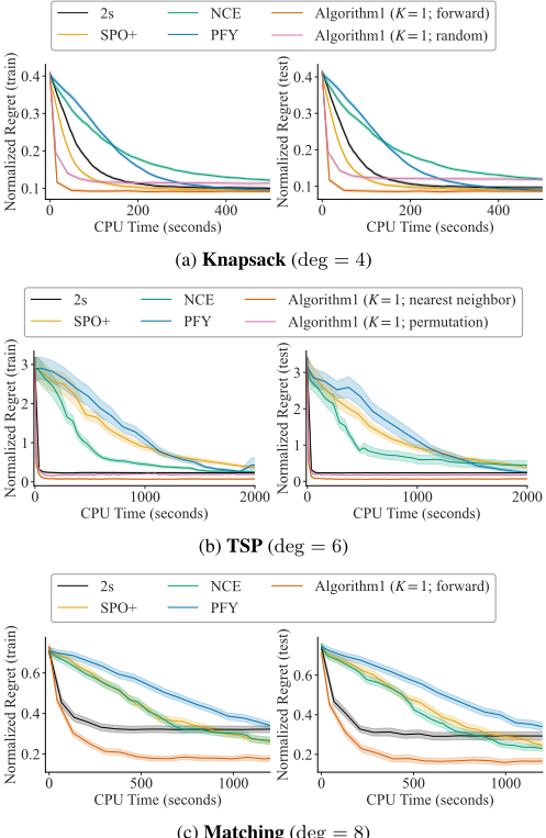
(c) Matching (deg = 8)
Figure 1: The learning curve of three contextual inverse optimization instances. The vertical axis represents the expected normalized regret on the training dataset (left) and the test dataset (right). The horizontal axis represents the execution time in seconds.
4.2 Synthetic Data Generation
The context vectors z ∈ Rd are generated from the normal distribution N(0d, Id), and we set d = 5 for all the experiments. For Knapsack instance, each entry of the objective coefficient vectors (ci)i is generated according to a polynomial mapping from the context vectors as ci = 5 3.5deg [([B∗z]i +3)deg +1] · εi, where deg > 0 is a predetermined polynomial degree, B∗ ∈ Rn×d is a latent true coefficient matrix whose each entry is generated from the Bernoulli distribution with mean 0.5, and εi is a multiplicative noise term generated from the uniform distribution on [1-ε, 1+ε] for some ε > 0. We denote the polynomial model as poly(z; B∗ , deg, ε). The weights of items, w = (wi)i, are sampled from {3, 4, . . . , 8} uniformly at random. Note that the data generation process based on the polynomial model is first employed in [Elmachtoub and Grigas, 2022] for the shortest path problem, and it has been used for other instances in subsequent research.
| Instance | 2s | SPO+ | NCE | PFY | Algorithm1(K = 1) | |||||
|---|---|---|---|---|---|---|---|---|---|---|
| (deg) | N-Reg | CPU[s/ep] | N-Reg | CPU[s/ep] | N-Reg | CPU[s/ep] | N-Reg | CPU[s/ep] | N-Reg | CPU[s/ep] |
| Knapsack (deg = 4) | 0.092 (0.028) | 0.06 (0.00) | 0.085 (0.026) | 0.97 (0.13) | 0.096 (0.028) | 1.37 (0.63) | 0.096 (0.026) | 1.27 (0.10) | 0.085 (0.026) | 21.78 (1.26) |
| TSP (deg = 6) | 0.224 (0.123) | 0.08 (0.01) | 0.214 (0.147) | 51.05 (1.28) | 0.268 (0.342) | 26.65 (13.38) | 0.084 (0.088) | 52.52 (1.36) | 0.065 (0.060) | 11.18 |
| 0.179 | 42.70 | (1.08) | ||||||||
| Matching = | 0.325 | 0.07 | 0.186 | 38.11 | 0.209 | 21.99 | 0.178 | 43.05 | ||
| (deg 8) | (0.156) | (0.02) | (0.121) | (6.00) | (0.131) | (11.82) | (0.120) | (1.87) | (0.121) | (1.01) |
For TSP instance, we generate cost matrix c = (cij)ij according to the same procedure as [Tang and Khalil, 2024, Sect. 5.1.3], which is based on the polynomial model defined by ck = 1 3deg -1 [ 1 √d [D∗z]k + 3]deg · ζk. Here, each element of the latent matrix D∗ is generated from the multiplication of Bernoulli distributions with mean 0.5 and uniform distribution on [-2, 2]. The noise term ζk is generated from the uniform distribution on [1 - ζ, 1 + ζ] for some ζ > 0. We denote this polynomial model as polyTSP(z; D∗ , deg, ζ).
For Matching instance, we generate a reward matrix according to the same polynomial model poly(z;B∗ , deg, ε) as the knapsack instance. The binary matrixm= (mij)ij is generated from Bernoulli distribution with mean 0.5.
The specific settings of parameters for the data generation process for each instance are described in the next subsection.
4.3 Experimental Setup
Baselines. For baselines, we compare the performance of the proposed algorithm with ridge regression as a standard two-stage method (2s) and SPO+ loss (SPO+) [Elmachtoub and Grigas, 2022] as existing methods for the completeinformation setting. We also employ the noise contrastive estimation method (NCE) [Mulamba et al., 2021] and perturbed Fenchel-Young loss (PFY) [Berthet et al., 2020] as existing methods for the incomplete-information setting. Note that the inverse optimization-based method proposed in [Hikima and Kamiyama, 2025] could, in principle, be applied under incomplete information; however, it requires solving inverse optimization at every iteration exactly. Preliminary experiments showed that applying this method to the problems considered in this section resulted in prohibitively high computational costs, so we exclude it from the comparison.
Implementation details. For all the experiments, we generate Ntr = 1024 and Nte = 1024 context-solution pairs for the training and test datasets, respectively. We use a linear model, h(z;Θ, θ0) = Θz + θ0, and train all the models by using stochastic gradient descent method [Amari, 1993] with a constant learning rate η = 5 · 10-3 and a mini-batch size of Ntr/4. We set the maximum number of epochs as T = 3 · 104 for the two-stage method and T = 100 for other methods.
Settings for the existing methods. For NCE method, we set the oracle-call ratio for solving the forward optimization to 0.5, and for PFY method, we set the number of perturbations as one and the perturbation level as 0.5. All the existing methods are implemented based on the Python-based PyEPO package [Tang and Khalil, 2024], which is an open-source software that supports modeling and solving optimization problems. Except for the two-stage approach, all the optimization problems are solved by using the GUROBI optimizer (version 12.0.3) [Gurobi Optimization, LLC, 2024].
Settings for the proposed method. Regarding the proposed method (Algorithm 1), we set K = 1, σ = 0.5, λ = 0, and T = 50. For the distance function in Eq. (2), we use the squared ℓ2-norm for Knapsack and TSP instances, and the ℓ1-norm for Matching instance. We report the ablation study on the number of samples K in Sect. 4.6. For sampling feasible solutions, we employed the forward sampling method described in Algorithm 1 and Algorithm 2 for Knapsack instance. For the TSP, we applied the nearest neighbor algorithm and the permutation-based sampling method as simple and practical choices. For the Matching, since no efficient sampling algorithm exists, we used the forward sampling method by solving the forward optimization problem with perturbed cost vectors. Similar to the existing methods, we model and solve the RIOP by using the CVXPY package and GUROBI optimizer (version 12.0.3).
Parameter settings for data generation ForKnapsack instance, we set n = 256, W = 512, and the polynomial model is set to be poly(z;B∗1 , 4, 0.75). For TSP instance, we set the number of cities as n = 16, and the polynomial model is set to be polyTSP(z;D∗ , 6, 0.5). For Matching instance, we set the number of nodes on each side as N1 = N2 = 10, and the polynomial model is set to be poly(z;B∗2 , 8, 1.0). Here, the latent matrix of each instance B∗i for i ∈ {1, 2} is generated from the Bernoulli distribution with mean 0.5, and D∗ is generated from the mixture of the Bernoulli distribution with mean 0.5 and the uniform distribution on [-2, 2].
4.4 EvaluationMetric
For one sample of the test data (z, c) ∈ Dte, we evaluate the performance of the existing methods and the proposed algorithm by the normalized regret, which is defined for a maximization problem as follows:
where h is a prediction model obtained by each algorithm. Using the test dataset Dte, we report the average and standard deviation of the normalized regret over all samples in Dte.
4.5 Comparison with ExistingMethods
Figure 1 shows the learning curves of the proposed algorithm and existing methods on each instance. The vertical axis represents the normalized regret on the training data (left), and test data (right), and the horizontal axis represents the execution time in seconds. The error bands represent an interval of one standard deviation above and below the mean. From the figure, we can see that the proposed algorithm reaches competitive regret values in a shorter wall-clock time than existing methods for all instances.
Table 1 shows the average and standard deviation of normalized regret on the test dataset based on the final model after training, and the average and standard deviation of execution time per epoch in seconds for each method. From the results, we can see that the proposed algorithm achieves comparable or better performance in terms of normalized regret compared to existing methods for all instances. For the Knapsack instance, our algorithm takes longer execution time per epoch compared to existing methods. This is likely because the knapsack problem is relatively easy to solve, allowing for faster computation than our algorithm, which requires solving the RIOP in Eq. (2) at each iteration.
In contrast, for the TSP instance, we can see that the proposed algorithm is more computationally efficient than existing methods. This is because, while other methods must solve the TSP exactly at each iteration, our algorithm solves the TSP approximately, thereby reducing the computational cost. Notice that the proposed algorithm repeatedly solves the RIOP to obtain the candidate coefficient parameters, but the RIOP with squared ℓ2-norm as the distance function can be formulated as a quadratic program, which can be solved efficiently with standard optimization solvers.
For theMatching instance, the computational time is comparable to existing methods because the proposed algorithm also solves a forward optimization problem to obtain feasible solutions. However, as can be confirmed in Figure 1, the proposed algorithm can achieve faster model training, and Table 1 shows comparable or better performance in terms of normalized regret.
Overall, these results (Figure 1 and Table 1) indicate that the proposed algorithm can effectively learn a prediction model for the contextual inverse optimization problems while maintaining computational efficiency.
4.6 Ablation Study on the Number of Samples K
To investigate the impact of the number of samples K on the performance of Algorithm 1, we conduct an ablation study by varying K. Table 2 reports the normalized regret on the test dataset and execution time per epoch for different K ∈ {1, 4, 16, 64} on the Knapsack and TSP instances. As sampling strategies in the proposed algorithm, we use Algorithm 2 and forward sampling method for the Knapsack instance, and the permutation-based sampling method and nearest neighbor algorithm for the TSP instance. The results indicate that even with K = 1, the proposed algorithm achieves performance comparable to that obtained with larger values of K. Moreover, the results suggest that higher-quality solutions generated through sampling lead to improved model performance, as reflected by lower normalized regret. However, a theoretical characterization of the relationship between the quality of sampled solutions and the performance of the proposed algorithm remains an open question.
4.7 Computational Complexity
The computational cost of existing methods is mainly governed by the number of times the forward optimization problem is solved. These methods typically require solving the forward optimization problem exactly at each iteration, either to evaluate the loss function or to obtain a gradient estimate for updating the model parameters. In contrast, when an efficient sampling method for generating feasible solutions is available, the proposed algorithm does not require solving the forward optimization exactly. In this case, the computational cost is mainly determined by the number of times the RIOP in Eq. (2) is solved. Thus, the main computational bottleneck shifts from repeatedly solving the forward optimization problem to repeatedly solving the RIOP. When no such sampling method is available, the proposed algorithm must also solve the forward optimization problem to generate feasible solutions, incurring additional computational cost compared with the case in which efficient sampling is available.
5 RelatedWork
This section reviews related work on CIO in which the available data are limited to context-solution pairs. For prior work on the complete-information setting, readers are referred to the survey papers [Sadana et al., 2024; Mandi et al., 2024].
5.1 Optimality Condition-Based Algorithm
[Sun et al., 2023] and [Mishra et al., 2024] proposed a method for learning the objective coefficients based on the optimality conditions for linear programs defined by minx {c⊤x ∣∣ Ax = b, x ≥ 0}, where A ∈ Rm×n and b ∈ Rm. For an arbitrary point q ∈ Rn and given optimal solution x⋆ , the algorithm in [Mishra et al., 2024] solves the quadratic program formulated as
where ν ∈ Rm and λ ∈ Rn≥0 are the Lagrange multipliers for the forward linear program, and the constraints are defined based on the KKT conditions of the linear program, which ensures that the given optimal solution x⋆ is optimal with respect to the optimal cost vector c for the above problem. Then, update the model parameters by minimizing the distance between the predicted cost vector and the optimal solution to the above quadratic program.
Both of the aforementioned methods rely on the optimality conditions of linear programs to update the prediction model, and their applicability is therefore restricted to settings in which such optimality conditions provide a tractable characterization of optimal solutions. In contrast, [Hikima and Kamiyama, 2025] proposed a more general framework that can be applied to a broad class of optimization with linear objective functions. Their method updates the prediction model by repeatedly solving an inverse optimization associated with the downstream optimization problem at each iteration.
| K = 1 | K = 4 | K = 16 | K = 64 | ||||||
|---|---|---|---|---|---|---|---|---|---|
| instance | sampler | N-Reg | CPU[s/ep] | N-Reg | CPU[s/ep] | N-Reg | CPU[s/ep] | N-Reg | CPU[s/ep] |
| Knapsack (deg = 4) | Algorithm 2 | 0.115 | 17.15 | 0.115 | 19.11 | 0.115 | 37.16 | 0.115 | 52.14 |
| (0.031) | (1.12) | (0.032) | (1.12) | (0.032) | (1.93) | (0.032) | (2.17) | ||
| forward | 0.085 | 21.78 | 0.085 | 39.46 | 0.085 | 102.44 | 0.084 | 323.33 | |
| (0.026) | (1.26) | (0.026) | (3.14) | (0.026) | (16.86) | (0.026) | (47.09) | ||
| TSP | permutation | 0.181 | 9.22 | 0.183 | 10.83 | 0.184 | 12.38 | 0.181 | 17.18 |
| (deg = 6) | (0.156) | (0.46) | (0.162) | (0.45) | (0.162) | (0.34) | (0.158) | (0.44) | |
| nearest neighbor | 0.065 | 10.56 | 0.062 | 11.28 | 0.063 | 13.84 | 0.063 | 22.73 | |
| (0.062) | (0.37) | (0.058) | (0.32) | (0.058) | (0.31) | (0.060) | (0.49) | ||
5.2 Perturbed Optimizer-Based Algorithm
[Berthet et al., 2020] proposed a learning algorithm for contextual inverse optimization problems based on the FenchelYoung loss framework [Blondel et al., 2020]. Given contextsolution pairs {(zi, xi)}Ni=1 ⊂ Rd × Rn , one can learn the prediction model h such that x⋆ε (h(zi)) ≈ xi, where x⋆ε (c) is a perturbed optimal solution defined as x⋆ε = Epc(x) [X] where pc(x) = P (x⋆ (c+εΞ) = x), and ε > 0 is a temperature parameter. Here Ξ ∈ Rn is a random variable with a positive and differentiable density dµ(ξ) ∝ exp(-ν(ξ))dξ. Unlike our approach, which constructs explicit regression targets by solving RIOP, the perturbed optimizer-based approach learns through a smoothed approximation of the optimizer induced by random perturbations. As observed in the experiments in Section 4, this difference leads to slower empirical convergence compared with our method.
5.3 AlgorithmBased on Enumerating Adjacent Solutions
[Berden et al., 2025] proposed a loss function called Loss via Adjacent Vertex Alignment which is defined for a hypothesis h ∈ H, and a data consisting of context z and an observed optimal solution x⋆ (c) ∈ X as
where Xadj(x) ⊂ X represents the set of vertices adjacent to x in the feasible region X, and ε ≥ 0 is a margin parameter. To train a prediction model based on the above loss function, it is required to enumerate all adjacent solutions for each observed solution. Therefore, [Berden et al., 2025] focus on linear programs where efficient methods based on performing pivots for enumerating adjacent vertices are known [Berthet et al., 2020; Gal and Geue, 1992]. On the other hand, for combinatorial optimization problems, it is generally difficult to enumerate all adjacent solutions efficiently. In particular, even for specific combinatorial optimization problems such as the {0, 1}-knapsack problem, there is no known efficient method for enumerating all adjacent feasible solutions. Furthermore, it is known that even determining whether two given vertices are adjacent is NP-complete [Matsui, 1995; Matsui and Tamura, 1995].
6 Conclusion
In conclusion, we have studied the contextual inverse optimization problem, which aims to learn a prediction model that estimates the unknown parameters of an underlying optimization problem from observed context-solution pairs. We have proposed an algorithm that iteratively solves a relaxed inverse optimization problem constructed based on feasible solutions sampled from the feasible region of the downstream optimization problem. The proposed algorithm can naturally incorporate a variety of sampling strategies for generating feasible solutions, making it applicable to a broad range of optimization problems. Numerical experiments demonstrate that our approach learns prediction models more efficiently than existing methods while achieving comparable or superior performance in terms of regret.
A limitation of the proposed framework is that its computational advantage relies on the availability of efficient methods for sampling feasible solutions. When such methods are unavailable, the forward optimization problem must be solved repeatedly to generate feasible solutions, which may reduce the computational benefits of the proposed approach. Another limitation is that the role of the sampled feasible solutions in the learning process is not yet theoretically characterized. The algorithm requires specifying the number of sampled feasible solutions, and the final performance of the model may depend not only on this number but also on the quality of the sampled solutions. Although our ablation study indicates that even one sampled solution can be sufficient in the tested instances and that higher-quality samples tend to yield better performance, clarifying how the number and quality of sampled feasible solutions affect the learned model remains an important direction for future research.
Acknowledgments
We thank the anonymous reviewers for their helpful comments and suggestions. This research was partially conducted by the Fujitsu Small Research Lab "Division of Fujitsu Mathematical Modeling for Decision Making," a joint research center between Fujitsu Limited andKyushuUniversity. In addition, this work was supported in part by JST ACT-X, Japan, Grant Number JPMJAX25CK, JST BOOST Program Grant Number JPMJBY24D1, and JSPS KAKENHI Grant Number JP26K21297.
@inproceedings{ijcai2026p484,
  title     = {A Sampling-Based Relaxation Approach to Contextual Inverse Optimization},
  author    = {Hikima, Yasunari and Kamiyama, Naoyuki and Sakaue, Shinsaku and Tsuchiya, Taira},
  booktitle = {Proceedings of the Thirty-Fifth International Joint Conference on
               Artificial Intelligence, {IJCAI-26}},
  publisher = {International Joint Conferences on Artificial Intelligence Organization},
  editor    = {Diego Calvanese},
  pages     = {4348--4357},
  year      = {2026},
  month     = {8},
  note      = {Main Track},
  doi       = {10.24963/ijcai.2026/484},
  url       = {https://doi.org/10.24963/ijcai.2026/484},
}
TY - CPAPER TI - A Sampling-Based Relaxation Approach to Contextual Inverse Optimization AU - Hikima, Yasunari AU - Kamiyama, Naoyuki AU - Sakaue, Shinsaku AU - Tsuchiya, Taira T2 - Proceedings of the Thirty-Fifth International Joint Conference on Artificial Intelligence, IJCAI-26 PB - International Joint Conferences on Artificial Intelligence Organization PY - 2026 SP - 4348 EP - 4357 DO - 10.24963/ijcai.2026/484 UR - https://doi.org/10.24963/ijcai.2026/484 ER -Copied
Machine-readable versions of this paper, for tools and AI agents:





