
Perturbation Matters in Time Series Forecasting: A Wave-attention-aware Transformer Method
Proceedings of the Thirty-Fifth International Joint Conference on Artificial Intelligence. Main Track. Pages 5012-5020.
https://doi.org/10.24963/ijcai.2026/558
Keywords
- Machine Learning: Time series and data streams
Abstract
Time series forecasting (TSF) refers to a fundamental task of predicting future sequential data based on historical observations. One representative category of TSF methods is transformer-based approaches, which translate time series into token sequences (i.e., as raw texts) before applying well-established transformers. In this paper, we conducted extensive preliminary experiments to evaluate their stability against various noises, and we empirically observed an interesting phenomenon: applying noises with appropriate levels to training time series can promote the predictive accuracy of transformer-based TSF methods. We analyze this phenomenon from the perspective of token attention and find one basic reason is that applying noises with appropriate levels can lead to token attention weights wavy, which is more consistent to the basic characteristic of time series data. Motivated by this phenomenon and analysis, we apply perturbations and propose a sub-objective wrt, perturbations constraining token attention weights to be wavy. Accordingly, we propose a novel TSF method, namely Wave-Attention-aware TransformER (WATER). We empirically evaluate \baby across the commonly used benchmark datasets, and experimental results indicate that it consistently outperforms the existing TSF methods.
- Method PatchTST (2023) WATER
- Crossformer (2023) WATER
- Metric MSE MAE MSE MAE MSE MAE MSE MAE ETTh1 96 0.377 0.397 0.366 0.394 0.411 0.435 0.394 0.419 192 0.409 0.425 0.407 0.419 0.409 0.438 0.404 0.430 336 0.431 0.444 0.429 0.442 0.433 0.457 0.425 0.451 720 0.457 0.477 0.455 0.475 0.501 0.514 0.486 0.501 ETTh2 96 0.274 0.337 0.274 0.337 0.728 0.603 0.722 0.607 192 0.348 0.384 0.344 0.383 0.723 0.607 0.712 0.601 336 0.377 0.416 0.372 0.409 0.740 0.628 0.738 0.627 720 0.406 0.441 0.395 0.432 1.386 0.882 1.332 0.854 ETTm1 96 0.289 0.343 0.287 0.343 0.314 0.367 0.319 0.362 192 0.329 0.368 0.326 0.367 0.374 0.410 0.360 0.400 336 0.362 0.390 0.358 0.387 0.413 0.432 0.398 0.427 720 0.413 0.423 0.412 0.420 0.753 0.613 0.720 0.582 ETTm2 96 0.165 0.255 0.163 0.254 0.296 0.391 0.282 0.378 192 0.221 0.293 0.221 0.292 0.369 0.416 0.325 0.392 336 0.276 0.327 0.271 0.333 0.588 0.600 0.498 0.510 720 0.362 0.381 0.361 0.381 0.750 0.612 0.750 0.612 References
- [Ahamed and Cheng, 2024] Md Atik Ahamed and Qiang Cheng. Timemachine: A time series is worth 4 mam- bas for long-term forecasting. In European Conference on Artificial Intelligence, volume 392, page 1688, 2024.
- [Box et al., 2015] George EP Box, Gwilym M Jenkins, Gre- gory C Reinsel, and Greta M Ljung. Time series analysis: forecasting and control. John Wiley & Sons, 2015.
- [Chen et al., 2024] Peng Chen, Yingying Zhang, Yunyao Cheng, Yang Shu, Yihang Wang, Qingsong Wen, Bin Yang, and Chenjuan Guo. Pathformer: Multi-scale transformers with adaptive pathways for time series forecasting. In Inter- national Conference on Learning Representations, 2024.
- [Cheng et al., 2024] Hao Cheng, Qingsong Wen, Yang Liu, and Liang Sun. Robusttsf: Towards theory and design of robust time series forecasting with anomalies. In Interna- tional Conference on Learning Representations, 2024.
- [Connor et al., 1994] Jerome T. Connor, R. Douglas Martin, and Les E. Atlas. Recurrent neural networks and robust time series prediction. IEEE Transactions on Neural Networks, 5(2):240-254, 1994.
- [Dai et al., 2024] Tao Dai, Beiliang Wu, Peiyuan Liu, Naiqi Li, Jigang Bao, Yong Jiang, and Shu-Tao Xia. Periodic- ity decoupling framework for long-term series forecasting. In International Conference on Learning Representations, 2024.
- [Deng et al., 2021] Jinliang Deng, Xiusi Chen, Renhe Jiang, Xuan Song, and Ivor W Tsang. St-norm: Spatial and tempo- ral normalization for multi-variate time series forecasting. In ACM SIGKDD Conference on Knowledge Discovery & Data Mining, pages 269-278, 2021.
- [Dietrich and Newsam, 1997] C. R. Dietrich and G. N. Newsam. Fast and exact simulation of stationary gaussian processes through circulant embedding of the covariance matrix. SIAM Journal on Scientific Computing, 18:1088- 1107, 1997.
- [Ghosh, 1996] M. Ghosh. Analysis of the effect of impulse noise on multicarrier and single carrier qam systems. IEEE Transactions on Communications, 44:145-147, 1996.
- [Goswami et al., 2023] Mononito Goswami, Cristian Ignacio Challu, Laurent Callot, Lenon Minorics, and Andrey Kan. Unsupervised model selection for time series anomaly de- tection. In International Conference on Learning Represen- tations, 2023.
- [Guo et al., 2023] Yong Guo, David Stutz, and Bernt Schiele. Robustifying token attention for vision transformers. In IEEE/CVF International Conference on Computer Vision, pages 17557-17568, 2023.
- [Hodrick and Prescott, 1997] Robert J. Hodrick and Ed- ward C. Prescott. Postwar u.s. business cycles: An empiri- cal investigation. Journal of Money, Credit and Banking, 29(1):1-16, 1997.
- [Kim et al., 2021] Taesung Kim, Jinhee Kim, Yunwon Tae, Cheonbok Park, Jang-Ho Choi, and Jaegul Choo. Re- versible instance normalization for accurate time-series forecasting against distribution shift. In International Con- ference on Learning Representations, 2021.
- [Kim et al., 2025] Jongseon Kim, Hyungjoon Kim, HyunGi Kim, Dongjun Lee, and Sungroh Yoon. A comprehensive survey of deep learning for time series forecasting: architec- tural diversity and open challenges. Artificial Intelligence Review, 58(7):216, 2025.
- [Kingma and Welling, 2014] Diederik P Kingma and Max Welling. Auto-encoding variational Bayes. In International Conference on Learning Representations, 2014.
- [Lai et al., 2021] Kwei-Herng Lai, Daochen Zha, Junjie Xu, Yue Zhao, Guanchu Wang, and Xia Hu. Revisiting time series outlier detection: Definitions and benchmarks. Ad- vances in Neural Information Processing Systems, pages 2117-2130, 2021.
- [Lin et al., 2024] Shengsheng Lin, Weiwei Lin, Xinyi Hu, Wentai Wu, Ruichao Mo, and Haocheng Zhong. Cyclenet: Enhancing time series forecasting through modeling peri- odic patterns. Advances in Neural Information Processing Systems, pages 106315-106345, 2024.
- [Liu et al., 2024] Yong Liu, Tengge Hu, Haoran Zhang, Haixu Wu, Shiyu Wang, Lintao Ma, and Mingsheng Long. itransformer: Inverted transformers are effective for time series forecasting. In International Conference on Learning Representations, 2024.
- [Ma et al., 2025] Jiaming Ma, Binwu Wang, Qihe Huang, Guanjun Wang, Pengkun Wang, Zhengyang Zhou, and Yang Wang. Mofo: Empowering long-term time series forecasting with periodic pattern modeling. Advances in Neural Information Processing Systems, 2025.
- [Mandelbrot and Ness, 1968] B. B. Mandelbrot and J. W. Van Ness. Fractional brownian motions, fractional noises and applications. SIAM Review, 10:422-437, 1968.
- [Mudelsee, 2019] Manfred Mudelsee. Trend analysis of cli- mate time series: A review of methods. Earth-science reviews, 190:310-322, 2019.
- [Nie et al., 2023] Yuqi Nie, Nam H Nguyen, Phanwadee Sinthong, and Jayant Kalagnanam. A time series is worth 64 words: Long-term forecasting with transformers. In In- ternational Conference on Learning Representations, 2023.
- [Obata et al., 2025] Kohei Obata, Yasuko Matsubara, and Ya- sushi Sakurai. Robust and explainable detector of time se- ries anomaly via augmenting multiclass pseudo-anomalies. In ACM SIGKDD Conference on Knowledge Discovery & Data Mining, pages 2198-2209, 2025.
- [Orvieto et al., 2022] Antonio Orvieto, Hans Kersting, Frank Proske, Francis Bach, and Aurelien Lucchi. Anticorre- lated noise injection for improved generalization. In Inter- national Conference on Machine Learning, pages 17094- 17116, 2022.
- [Percival and Walden, 2000] D. B. Percival and A. T. Walden. Wavelet Methods for Time Series Analysis, volume 4. Cam- bridge university press, 2000.
- [Pighi et al., 2009] R. Pighi, M. Franceschini, G. Ferrari, and R. Raheli. Fundamental performance limits of communica- tions systems impaired by impulse noise. IEEE Transac- tions on Communications, 57:171-182, 2009.
- [Qiu et al., 2024] Xiangfei Qiu, Jilin Hu, Lekui Zhou, Xingjian Wu, Junyang Du, Buang Zhang, Chenjuan Guo, Aoying Zhou, Christian S Jensen, Zhenli Sheng, et al. Tfb: Towards comprehensive and fair benchmarking of time series forecasting methods. VLDB Endowment, 17(9):2363- 2377, 2024.
- [Rouphael, 2014] T. J. Rouphael. Wireless Receiver Archi- tectures and Design: Antennas, RF, Synthesizers, Mixed Signal and Digital Signal Processing. Academic Press, 2014.
- [Shongwe et al., 2014] T. Shongwe, A. H. Vinck, and H. C. Ferreira. On impulse noise and its models. In IEEE Inter- national Symposium on Power Line Communications and Its Applications, pages 12-17, 2014.
- [Snyder and Miller, 1991] Donald L Snyder and Michael I Miller. Random point processes in time and space. Springer New York, 1991.
- [Theodorsen et al., 2017] A. Theodorsen, O. E. Garcia, and M. Rypdal. Statistical properties of a filtered poisson pro- cess with additive random noise: distributions, correlations and moment estimation. Physica Scripta, 92(5):054002, 2017.
- [Tsihrintzis and Nikias, 1995] G. A. Tsihrintzis and C. L. Nikias. Performance of optimum and suboptimum receivers in the presence of impulsive noise modeled as an alpha- stable process. IEEE Transactions on Communications, 43:904-914, 1995.
- [Vasilescu, 2006] G. Vasilescu. Electronic Noise and Interfer- ing Signals: Principles and Applications. Springer Science & Business Media, 2006.
- [Wang et al., 2024a] Shiyu Wang, Haixu Wu, Xiaoming Shi, Tengge Hu, Huakun Luo, Lintao Ma, James Zhang, and JUN ZHOU. Timemixer: Decomposable multiscale mixing for time series forecasting. In International Conference on Learning Representations, pages 38626-38652, 2024.
- [Wang et al., 2024b] Yuxuan Wang, Haixu Wu, Jiaxiang Dong, Guo Qin, Haoran Zhang, Yong Liu, Yunzhong Qiu, Jianmin Wang, and Mingsheng Long. Timexer: Empower- ing transformers for time series forecasting with exogenous variables. Advances in Neural Information Processing Sys- tems, 37:469-498, 2024.
- [Wang et al., 2025a] Bing Wang, Ximing Li, Yiming Wang, Changchun Li, Jiaxu Cui, Renchu Guan, and Bo Yang. Va- riety is the spice of life: Detecting misinformation with dynamic environmental representations. In ACM Interna- tional Conference on Information and Knowledge Manage- ment, pages 2945-2955, 2025.
- [Wang et al., 2025b] Zihan Wang, Fanheng Kong, Shi Feng, Ming Wang, Xiaocui Yang, Han Zhao, Daling Wang, and Yifei Zhang. Is mamba effective for time series forecasting? Neurocomputing, 619:129178, 2025.
- [Wu et al., 2021] Haixu Wu, Jiehui Xu, Jianmin Wang, and Mingsheng Long. Autoformer: Decomposition transform- ers with auto-correlation for long-term series forecast- ing. Advances in Neural Information Processing Systems, 34:22419-22430, 2021.
- [Wunderlich and Sklar, 2023] Adam Wunderlich and Jack Sklar. Data-driven modeling of noise time series with convolutional generative adversarial networks. Machine Learning: Science and Technology, 4(3):035023, 2023.
- [Xiao et al., 2024] Guangxuan Xiao, Yuandong Tian, Beidi Chen, Song Han, and Mike Lewis. Efficient streaming language models with attention sinks. In International Conference on Learning Representations, volume 2024, pages 21875-21895, 2024.
- [Yang et al., 2025] Chen Yang, Yangfan He, Aaron Xuxiang Tian, Dong Chen, Jianhui Wang, Tianyu Shi, Arsalan Hey- darian, and Pei Liu. Wcdt: World-centric diffusion trans- former for traffic scene generation. In IEEE International Conference on Robotics and Automation, pages 6566-6572, 2025.
- [Yin et al., 2025] Zhengwei Yin, Hongjun Wang, Guixu Lin, Weihang Ran, and Yinqiang Zheng. Random is all you need: Random noise injection on feature statistics for generaliz- able deep image denoising. In International Conference on Learning Representations, 2025.
- [Yoon et al., 2022] TaeHo Yoon, Youngsuk Park, Ernest K Ryu, and Yuyang Wang. Robust probabilistic time series forecasting. In International Conference on Artificial Intel- ligence and Statistics, pages 1336-1358, 2022.
- [Zeng et al., 2023] Ailing Zeng, Muxi Chen, Lei Zhang, and Qiang Xu. Are transformers effective for time series fore- casting? In AAAI Conference on Artificial Intelligence, volume 37, pages 11121-11128, 2023.
- [Zhang and Yan, 2023] Yunhao Zhang and Junchi Yan. Cross- former: Transformer utilizing cross-dimension dependency for multivariate time series forecasting. In International Conference on Learning Representations, 2023.
- [Zhou et al., 2021] Haoyi Zhou, Shanghang Zhang, Jieqi Peng, Shuai Zhang, Jianxin Li, Hui Xiong, and Wancai Zhang. Informer: Beyond efficient transformer for long se- quence time-series forecasting. In AAAI Conference on Ar- tificial Intelligence, volume 35, pages 11106-11115, 2021.
- [Zhou et al., 2022] Tian Zhou, Ziqing Ma, Qingsong Wen, Xue Wang, Liang Sun, and Rong Jin. Fedformer: Fre- quency enhanced decomposed transformer for long-term series forecasting. In International Conference on Machine Learning, pages 27268-27286, 2022.
References were extracted automatically from the PDF and may contain errors.
Full text extracted automatically from the PDF; figures, tables and equations may differ. The PDF is the version of record.
1 Introduction
Time Series Forecasting (TSF) refers to the task of predicting future sequential data based on historical observations [Qiu et al., 2024; Kim et al., 2025]. As a fundamental task of machine learning, it has been widely adopted in many real-world applications, such as climate forecasting, epidemic analysis, energy management, financial investment, and traffic planning [Mudelsee, 2019; Deng et al., 2021; Yang et al., 2025; Wang et al., 2025a].
During the past decades, many TSF methods have been developed [Zeng et al., 2023; Ahamed and Cheng, 2024;
∗Corresponding author
Wang et al., 2025b]. Transformer-based TSF methods have recently attracted much attention because of their high performance, especially for long-term forecasting [Nie et al., 2023; Zhang and Yan, 2023; Liu et al., 2024]. Technically, they follow the spirit of problem transformation, whose basic idea is to translate time series into token sequences (i.e. as raw texts) before applying well-established transformers. For example, PatchTST, a representative transformer-based TSF method, applies the patching technique to group segments of time series into tokens [Nie et al., 2023]. In contrast, iTransformer treats each time series of a variate as a single token and models inter-variate dependencies by attention [Liu et al., 2024]. Regarding the attention-based dependency modeling, a simpleyet-effective approach is to treat each variate independently and model the temporal dependencies using attention [Nie et al., 2023]. Building on this, Crossformer introduces a Two-Stage Attention mechanism to simultaneously capture both cross-time and cross-dimension dependencies [Zhang and Yan, 2023], and Pathformer integrates the modeling of intra-dependencies within each token.
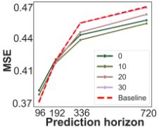
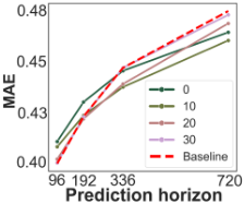
Our initial research intention is to investigate the effectiveness of transformer-based TSF methods in various scenarios, and in this paper, our story begins with the empirical study of their stability against noises. Specifically, we apply 4 benchmark time series datasets. For each one, we inject 2 types of noise with different levels (in total 160+ settings) into the training data, and separately train PatchTST models with them. We then evaluate the forecasting performance on test data to analyze how stable it is with different noises and levels. We surprisingly find that, in most cases, injecting noise with appropriate levels can effectively boost the forecasting performance, especially on the longer horizons (see Fig. 1). This phenomena naturally raises the question: why does injecting noises with appropriate levels lead to such a pronounced improvement in time series forecasting?
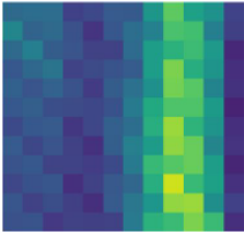
To explore the underlying reasons, we investigate the token attention weights in transformers, i.e. the critical component to extract temporal dependencies. Interestingly, we observe that noise injection at an appropriate level makes the attention weights exhibit a wave-like pattern, rather than being concentrated on a small set of tokens (see Fig 2). Comparing with highly concentrated attention weights, the wavy attentions may reflect the intrinsic characteristics of time series data, such as temporal continuity, periodicity and multi-scale dependencies, yielding more informative representations to improve the forecasting performance.
Inspired by this phenomena, we propose a novel TSF method to adaptively perturb the training data which constrains the token attention weights to be wavy, namely WaveAttention-aware TransformER (WATER). Specifically, we apply Gaussian perturbations with zero mean and a learnable standard deviation (std) parameter to control the perturbation level. We optimize std parameters by maximizing the secondorder differences on the attention weights of each token. In this way, each token attention weight is encouraged to have locally high-curvature structures and thereby exhibiting a wave-like pattern, rather than highly concentrated on a small set of tokens. By constraining the token attention weights to be wavy, our WATER can adaptively learn perturbations at an appropriate level, which can induce richer temporal dependencies and consequently more informative token representations to promote forecasting performance. In a nutshell, our contributions are summarized as below:
- We conduct extensive preliminary studies on transformerbased TSF methods to evaluate the stability over various noise types. We surprisingly find that appropriate noise levels can promote the forecasting performance and make the token attention weights wavy.
- Inspired by the above phenomena, we propose a novel TSF method WATER which adaptively perturbs the training data by constraining the token attention weights to be wavy via maximizing the corresponding second-order differences.
- We examine WATER by several time series forecasting tasks against SOTA baseline methods on benchmark datasets. And the experimental results demonstrate that our WATER can achieve effective performance improvements.
2 Preliminary Study
We conduct preliminary experiments to evaluate how transformer-based TSF methods are stable with different noises and levels.
2.1 Settings
In this preliminary study, we apply PatchTST because it is acknowledged as a classic transformer-based TSF method. Specifically, we collect 4 benchmark time series datasets (ETTh1, ETTh2, ETTm1, ETTm2), and for each one, we inject noises into the training data. We then train PatchTST with them, and our goal is to evaluate the performance differences on test data between the models trained with and without noises.
We apply 2 types of noises, i.e. structure-agnostic and structure-aware noises, with different levels, totally collecting 160+ settings. Specifically, for structure-agnostic noises, we adopt Gaussian noise, power law noise (Fractional Gaussian noise, FGN), shot noise and impulsive noise (BernoulliGaussian noise, BG) following [Wunderlich and Sklar, 2023]. Noise levels are controlled by varying the signal-to-noise
- (a) Train w/ Gauss. noise.
(b) Train w/ FGN noise.
Figure 1: The MSE and MAE scores of PatchTST on dataset ETTh1 when applying Gaussian and FGN noises with different levels (SNR={0, 10, 20, 30} dB) on training data.
rate (SNR) from {-5, 0, 5, 10, 15, 20, 25, 30} dB and noisespecific parameters, e.g. the Bernoulli mask probability for controlling whether to add Gaussian noise on each time point is set as {0.1, 0.5, 0.7, 1.0}. For structure-aware noises, we adopt Speedup, Cutoff and Scaling transformations following [Obata et al., 2025]. The noise levels are controlled by varying mask ratios from {0.01, 0.1, 0.2, . . . , 0.7}, which controls the proportion of a sequence to be transformed, and scaling parameters from {0.01, 1.0, 2.0, 3.0, 4.0}, which controls noise scaling in noise addition. Statistics of datasets are presented in Table 4 in Appendix. Detailed noise additions and parameter settings are presented in Appendix B.1 and Table 5.
2.2 Empirical Observations
We report the averaged MSE/MAE scores of applying Gaussian and FGN noises on ETTh1 over different historical sequence lengths in Fig. 1a, 1b and full results of different noises are presented in Appendix B.2.
We can surprisingly find that applying noise at appropriate levels can effectively promote the forecasting performance, especially for longer horizons. As the noise level gradually increases frommild to excessive, the overall forecasting performance gain first increases and then deteriorates, and are more significant when horizon=336/720. Specifically, an appropriate noise here refers to noise that slightly blurs local details without altering the overall trend (e.g. the corrupted series with Gaussian noise of 15 dB in Fig. 6). Such noises typically happens at SNR ∈ {15, 20, 25} dB.
2.3 Analysis from Self-Attention Perspective
To explore the underlying reason, we investigate the effect of noise on the token attention weights, which are crucial for modeling complex temporal dependencies in transformerbased methods. We focus on 4 structure-agnostic noises and compare token attention weights between training with and without applying noises on ETTh1 and present a toy attention comparison in Fig. 2. More results of token attention weights are presented in Figs. 18, 19, 20, 21 in Appendix B.2. We can find that applying noise to training data makes the token attention weights wavy and effectively mitigates the extremetoken phenomena.
When training without noise, the extreme-token phenomena is relatively severer than training with noise, i.e. higher attention weights are concentrated on a small set of tokens,
- (a) Train w/o noise.
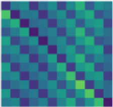
Figure 2: Output token attention weights comparing training without noise and training with applying Gaussian noise of SNR=20 dB.
and the rest tokens receive only negligible weights. This is a common issue in transformer-based methods and has been widely discussed in previous studies [Guo et al., 2023; Xiao et al., 2024]. Such attention pattern contradicts the complex temporal dependency nature of time series data. It may result in collapsed and less discriminative token representations, thereby harming the overall forecasting performance.
When training with noise, the token attention weights become wavier, where the attention weights of each token vary with temporal distance and exhibiting a rising-or-falling local pattern in a non-monotonic manner. This wave-like pattern may suggest that applying noise encourages the model to aggregate information across different temporal ranges and can effectively explore the intrinsic characteristics of time series data, such as local continuity, periodicity, and multi-scale temporal dependencies. Therefore, the induced attention weights becomes more consistent with the complex characteristics of time series data, leading to more informative token representations and improved forecasting performance.
In a word, applying noise to training data with appropriate levels can induce a wave-like token attention weights, which may reflect the intrinsic characteristics of time series data. This inspires us to adaptively introduce perturbations by constraining the token attention weights to be wavy, thereby improving the overall forecasting performance.
3 Method
For simplicity of notations, we introduce our method from the perspective of univariate time series forecasting. We denote an observed time series sequence by xi = [xi,0, xi,2, . . . , xi,L-1]⊤ ∈ RL, where L denotes the historical sequence length. The time series forecasting task aims at predicting the future sequence yi = [yi,0, yi,2, . . . , yi,F-1]⊤ ∈ RF of length F. Generally, we collect a set of N times series D = {(xi, yi)}Ni=1 as training data to learn a forecasting model f(·) which can accurately predict the future sequence using the observed time series.
Inspired by the preliminary experiments, we propose a novel TSF method WATER to perturb the training data to enhance the overall predicting performance. To induce an appropriate perturbation level, we introduce a second-order difference maximization constraint to encourage the token attention weights to be wavy. We will introduce the details of WATER in the following.
3.1 Learnable Gaussian Perturbations
We consider the Gaussian perturbations and control the noise level by a learnable parameter of standard deviation (std). Specifically, for sequence xi, to exert noise with different levels on each time point, we set the std parameter as σi ∈ RL and the perturbed input is given by:
where ei denotes the Gaussian perturbations and is calculated by the reparameterization trick [Kingma and Welling, 2014]:
The standard deviation parameter is optimized by encouraging the model to output a wavy token attention matrix along with model training, which will be introduced in the following.
3.2 Tokenization and Forecasting
We adopt a transformer-based TSF method which considers token-wise attentions to predict the future sequence ˆyi. We first pre-process the perturbed sequence by Instance Normalization [Kim et al., 2021] and then patch it into several tokens to adapt the input formats of transformers. Specifically, each perturbed sequence ˜x ∈ RH is patched into xi = [xi,1, . . . , xi,Ps ] ∈ RLp×Ps , where xi,j = [˜xi,(j-1)·Lp+1, . . . , ˜xi,j·Lp ]⊤ ∈ RLp denotes the jth token; Lp denotes the token length; Ps = ⌊L/Lp⌋ + 2 denotes the number of patches.
Then we adopt an embedding layer fWe (·), C stacked transformer layers fW1:C t (·) and a flatten-linear predictor fWf (·) to predict the future sequence ˆyi:
We learn the model by optimizing the objective:
where ℓ(·, ·) denote the forecasting loss and we adopt the weighted loss following [Ma et al., 2025].
3.3 Wavy Attention Constraint
Taking inspiration from preliminary studies showing that appropriate noise injection yields wave-like token attention patterns, we adaptively learn input perturbations by directly maximizing the second-order difference of token attention weights to encourage higher curvature.
Specifically, for each token sequence xi, its corresponding attention weight across all tokens is denoted by Ai = {Ac,h i }, where Ac,h i ∈ RLp×Lp , c ∈ [1,C] denotes the transformer layer index and h ∈ [1,H] denotes the attention head index. Specially, it's worth mentioning that the attention matrix Ac,h i can be derived from various attention mechanisms across different backbones, making our method generalizable to any transformer-based TSF model that considers token-wise attention. To induce wavy token attention weights, inspired by [Hodrick and Prescott, 1997], we introduce a second-order difference maximization constraint on the attention weight Algorithm 1 Training procedure of WATER.
Input: Time series data {(xi, yi)}Ni=1 Output: Optimal parameters {σ∗ ,W∗ e , W1:C t ∗ , W∗ f } of
WATER
- 1: Initialize {σ,We,W1:C t ,Wf};
- 2: for epoch e = 1 toMaxEpoch do
- 3: for iter it = 1 to MaxIter do
- 4: Add Gaussian perturbations to each xi by Eq. (1);
- 5: Calculate the training objective of Eq. (6);
- 6: Update {σ,We,W1:C t ,Wf} by back-propagation;
- 7: end for
- 8: end for
distribution of each token to induce higher curvature on each token. Therefore, we set the following maximization objective:
where ∆2 ((Ac,h i )j,k) denotes the second-order difference of Ac,h i along k.
In this way, the local curvatures of each token point are encouraged to be higher, thereby promoting a wave-like pattern in the overall token attention matrix. Each token are encouraged to attend to more tokens across different temporal ranges, which is consistent with the intrinsic data characteristics of time series, such as local continuity, multiple periodicity, etc. In this way, we can utilize more complex temporal dependencies to induce more informative token representations, which contributes to promoted forecasting performance.
By combining the above two objectives, the whole learning objective is formulated as below:
where λ denotes the scaling parameter, A = {Ai}Ni=1 denotes the set of token attentions of all samples. By optimizing the above objective, we can adaptively learn the standard deviation parameter by constraining the token attention weights to be wavy, thereby adaptively adding noise to the input series, further promoting the overall forecasting performance. The overall model training process of WATER is summarized in Algorithm 1.
4 RelatedWork
4.1 Time Series Forecasting
In the past decades, time series forecasting methods have evolved from statistical techniques, such as exponential smoothing and ARIMA models [Box et al., 2015], to advanced machine learning approaches. Recently, deep learning methods have been widely adopted to capture complex temporal patterns, such as MLP, RNN, CNN, Transformers, diffusion models and Mamba, etc.
Transformers has been widely adopted for TSF due to excelling at capturing long-term dependencies. However, early point-wise transformers-based TSF methods suffer from quadratic computational complexity. To address this problem, researchers have devoted into several directions, including sparsity decomposition, tokenization, etc. Informer [Zhou et al., 2021] treats each time series as a single token and models variable dependencies using attention mechanisms. Building upon this paradigm, models such as Autoformer [Wu et al., 2021] and FEDformer [Zhou et al., 2022] successfully reduced complexity using sparsity strategies. More recently, researches integrate tokenization technique to induce tokenwise methods, which significantly reduce the computational complexity and adapt transformers for modeling longer sequences. PatchTST [Nie et al., 2023] is one of the pioneers which adopts the simple channel independency assumption. Crossformer [Zhang and Yan, 2023] develops a two-stage attention mechanism to simultaneously capture the inter- and intra-variate dependencies. Pathformer [Chen et al., 2024] propose to segment time series into patches of different sizes and use a multi-scale router to extract temporal dependencies frommultiple resolutions. TimeXer [Wang et al., 2024b] introduced variable-level tokens to account for bidirectional dependencies.
Building upon transformer-based TSF methods, our work observes that injecting noise at an appropriate level into the input time series consistently improves forecasting performance. Motivated by this, we propose WATER, which adaptively learns the perturbation level by encouraging the token-wise attention weights to be wavy, thereby enabling richer temporal dependencies and promoting the forecasting performance.
4.2 Performance Enhancement via Perturbations
In the machine learning community, introducing controlled perturbations during training has been widely adopted as an effective approach to improve model generalizability and robustness. A prevalent way is to design artificial noise injection as implicit regularizer, which leads into smoother solutions and effectively alleviates overfitting [Orvieto et al., 2022]. In computer vision, [Yin et al., 2025] applies random noise into feature statistics within the model. This strategy significantly improves generalization under unseen noise distributions. Similar ideas have also been explored in TSF. For example, [Yoon et al., 2022] introduces noise during training to achieve certified robustness against bounded adversarial perturbations. [Cheng et al., 2024] systematically studies the effects of different anomaly injection strategies on TSF. Based on their findings, they propose a robust forecasting framework. Overall speaking, injecting noise into training data can enhance the model generalization, leading to more robust and accurate prediction performance.
| Method | WATER (Ours) | MoFo (2025) | PDF (2024) | iTransformer (2024) | Pathformer (2024) | CycleNet (2024) TimeMixer (2024) | PatchTST (2023) | Crossformer (2023) | DLinear (2023) | |||||||||||||||
|---|---|---|---|---|---|---|---|---|---|---|---|---|---|---|---|---|---|---|---|---|---|---|---|---|
| Metric | MSE | MAE | MSE | MAE | MSE | MAE | MSE | MAE | MSE MAE | MSE | MAE | MSE | MAE | MSE | MAE | MAE | MSE | MAE | ||||||
| ETTh1 | 96 192 336 | 0.357↑0.83% 0.395↓0.77% 0.407↑1.93% 0.427↑4.69% | 0.389↑0.51% 0.415↓0.24% 0.428↑0.23% 0.449↑1.97% | 0.363 0.407 0.415 0.449 | 0.392 0.420 0.429 0.458 | 0.360 0.392 0.418 0.456 | 0.391 0.414 0.435 | 0.386 0.424 0.449 | 0.405 0.440 0.460 | 0.372 0.392 0.408 0.415 0.438 0.434 | 0.372 0.404 0.430 | 0.394 0.417 0.429 0.448 0.464 | 0.372 0.413 0.438 0.486 | 0.484 | 0.401 0.430 0.450 | 0.377 0.397 0.409 0.425 0.431 0.444 | 0.411 0.409 0.433 0.501 | 0.435 0.438 0.457 0.514 | 0.379 0.408 0.440 0.471 | 0.403 0.419 0.440 | ||||
| ETTh2 | 720 96 192 336 720 | 0.272↑0.73% 0.327↑1.51% 0.377↑2.58% | 0.325↑0.61% 0.375↑1.06% 0.351↑3.04% 0.398↑1.97% 0.421↑2.09% | 0.278 0.332 0.362 0.387 | 0.327 0.379 0.406 0.430 | 0.276 0.339 0.374 0.398 | 0.462 0.341 0.382 0.406 0.433 | 0.495 0.297 0.372 0.388 0.424 | 0.487 0.348 0.403 0.417 0.444 | 0.450 0.463 0.279 0.336 0.345 0.380 0.378 0.408 | 0.277 0.341 0.370 | 0.341 0.385 0.411 0.424 | 0.281 0.349 0.366 0.451 0.401 | 0.351 0.387 0.413 0.436 | 0.457 0.274 0.348 0.377 | 0.477 0.337 0.384 | 0.728 0.723 0.740 | 0.603 0.607 0.628 0.882 | 0.300 0.387 0.490 0.704 | 0.493 0.364 0.423 0.487 0.597 | ||||
| ETTm1 | 96 192 336 720 | 0.279↑1.76% 0.320↑0.31% 0.350↑1.13% 0.396↑2.46% | 0.336↓0.30% 0.361↑0.55% 0.386↓0.78% 0.413↓0.24% 0.243↑0.41% 0.280↑1.75% | 0.284 0.326 0.354 0.406 0.156 | 0.336 0.364 0.384 0.417 0.244 0.285 0.317 | 0.286 0.321 0.354 0.408 0.163 0.219 0.269 0.349 0.147 0.193 | 0.340 0.364 0.383 0.415 0.251 0.290 0.330 0.382 | 0.300 0.341 0.374 0.429 0.175 0.242 0.282 | 0.353 0.380 0.396 0.430 0.266 | 0.437 0.290 0.337 0.374 0.428 | 0.455 0.335 0.363 0.384 0.416 0.250 | 0.297 0.332 0.365 0.366 0.386 0.417 0.414 0.247 | 0.344 0.293 0.335 0.365 0.426 0.165 0.225 | 0.345 0.372 0.386 0.412 0.256 | 0.406 0.289 0.329 0.362 0.413 0.165 0.221 | 0.416 0.441 0.343 0.368 0.390 0.423 0.255 0.293 | 1.386 0.314 0.374 0.413 0.753 0.296 | 0.367 0.410 0.432 0.613 | 0.300 0.336 0.367 0.419 0.164 | 0.345 0.366 0.386 0.416 | ||||
| ETTm2 | 96 192 336 720 | 0.155↑0.64% 0.208↑2.80% 0.259↑2.63% 0.344↑1.15% | 0.314↑0.95% 0.370↑0.27% | 0.214 0.266 | 0.348 | 0.371 0.245 | 0.375 | 0.312 0.337 0.394 | 0.164 0.219 0.267 0.361 | 0.288 0.319 0.377 0.195 | 0.157 0.214 0.286 0.269 0.322 0.363 0.382 | 0.277 0.360 0.147 | 0.298 0.332 0.387 0.198 | 0.276 0.362 0.150 0.191 | 0.327 0.381 0.200 0.239 0.279 0.330 | 0.750 0.143 0.195 0.254 | 0.391 0.416 0.600 0.612 | 0.224 0.277 0.371 0.170 | 0.255 0.304 0.337 0.401 | 0.369 0.588 | ||||
| 96 192 336 720 96 | 0.139↑1.42% 0.183↑1.61% 0.234↓0.43% 0.307↑1.60% | 0.141 0.186 0.233 | 0.186 0.231 0.271 0.330 | 0.196 0.240 0.280 0.323 0.334 | 0.157 0.200 0.252 0.320 | 0.207 0.248 0.287 0.336 | 0.148 0.191 0.243 | 0.166 0.235 0.274 0.326 | 0.213 0.262 0.329 | 0.222 0.259 0.192 0.291 0.247 0.338 0.318 | 0.243 0.284 0.330 0.232 | 0.242 0.312 | 0.234 0.302 0.293 | 0.335 0.183 0.208 0.212 0.215 | 0.210 0.261 0.319 0.385 | 0.216 0.258 0.323 | 0.230 0.273 0.307 0.362 | |||||||
| Weather | 0.184↑1.08% 0.229↑0.87% 0.269↑0.74% | 0.313 0.172 0.176 0.186 | 0.210 0.229 0.244 0.244 | 0.247 0.257 0.269 | 0.190 0.193 0.203 | 0.244 0.257 0.266 | 0.318 0.218 | 0.235 0.220 0.220 | 0.252 0.261 0.269 | 0.170 0.204 0.212 0.215 | 0.307 | 0.208 0.226 0.239 0.256 | 0.199 | |||||||||||
| Solar | 192 336 720 0.191↑1.55% | 0.338↓3.68% 0.205↑1.44% 0.226↓2.73% 0.234↓6.36% 0.241↓1.69% | 0.194 | 0.181 0.199 0.208 0.212 | 0.223 | 0.179 | 0.259 0.256 0.261 | 0.143 0.158 | 0.247 0.260 | |||||||||||||||
| 0.161↑5.29% 0.171↑2.84% 0.180↑3.23% | 0.130 | 0.224 0.239 | 0.275 0.222 | 0.281 | 0.196 0.195 0.208 | 0.201 0.221 0.233 0.236 | 0.271 | 0.201 0.190 0.203 | 0.256 | 0.168 | 0.220 0.234 0.243 | 0.265 0.282 0.295 | ||||||||||||
| 0.126↑1.56% | 0.219↑0.90% 0.235↑1.67% 0.253↑0.78% 0.284↑0.70% | 0.146 0.161 0.200 | 0.255 | 0.128 0.147 | 0.134 0.154 0.169 | 0.230 0.250 0.265 0.288 | 0.237 0.135 0.157 0.170 | 0.126 0.144 0.161 | 0.221 0.239 0.253 | 0.153 0.168 0.189 0.228 | 0.269 | 0.214 | 0.267 | 0.134 0.146 0.165 | 0.154 0.169 0.204 | 0.301 | 0.140 | |||||||
| Electricity | 96 192 336 720 | 0.143↑0.69% 0.158↑1.86% 0.192↑1.03% | 0.375 | 0.290 0.254 | 0.165 0.199 | 0.242 0.260 0.289 | 0.194 | 0.222 0.253 0.267 0.211 | 0.199 0.389 | 0.286 0.276 | 0.369 | 0.291 0.320 | 0.307 | 0.237 | 0.231 0.243 0.264 | 0.395 | 0.237 0.251 0.268 | |||||||
| 96 | 0.374↓3.03% | 0.254↓1.60% 0.261↓1.56% | 0.388 | 0.261 | 0.368 | 0.252 0.261 | 0.363 | 0.265 0.273 | 0.302 0.384 0.250 | 0.406 | 0.280 | 0.400 | 0.257 0.272 | 0.370 0.386 | 0.262 0.269 | 0.526 0.503 | 0.314 0.288 0.263 | 0.301 0.275 | ||||||
| 0.400 | 0.268 | 0.277 | 0.405 0.424 | 0.425 | 0.275 | 0.276 | 0.280 | |||||||||||||||||
| 0.389↓1.83% 0.399↓1.53% | 0.269↓1.51% | 0.382 | 0.384 0.396 | 0.291 | 0.407 | |||||||||||||||||||
| Traffic | 192 336 | 0.257 | 0.396 | |||||||||||||||||||||
| 0.393 | 0.268 | 0.308 | 0.417 0.454 | 0.286 0.308 | 0.505 | |||||||||||||||||||
| 720 | 0.435 | 0.289 | 0.438 | 0.297 | 0.265 0.283 | 0.407 | 0.272 0.316 | 0.295 | ||||||||||||||||
| 0.289↓2.12% | 0.450 | 0.303 | 0.435 | 0.552 | 0.301 | |||||||||||||||||||
| 0.445 | ||||||||||||||||||||||||
| 0.461 | ||||||||||||||||||||||||
| 0.435↑0.68% | 0.452 | |||||||||||||||||||||||
5 Experiment
5.1 Experimental Settings
Datasets
We conduct our experiments on 8 benchmark time series datasets, including ETTh1, ETTh2, ETTm1, ETTm2, Weather, Solar Energy, Electricity, and Traffic [Zhou et al., 2021]. Statistics are summarized in Table 4.
Baseline Methods
We compare WATER with 9 advanced time series forecasting methods as baselines, comprising MoFo [Ma et al., 2025], PDF [Dai et al., 2024], iTransformer [Liu et al., 2024], Pathformer [Chen et al., 2024], CycleNet [Lin et al., 2024], TimeMixer [Wang et al., 2024a], PatchTST [Nie et al., 2023], Crossformer [Zhang and Yan, 2023] and DLinear [Zeng et al., 2023].
Implementation Settings
We adopt MoFo [Ma et al., 2025] as the backbone forecasting model and set the periodic length as 24. We also evaluate our WATER on other transformer-based backbones which consider token-wise attentions in latter sections. Each σi is initialized by exp(-2.0). The initial learning rate is set as 0.01 and we decay it by half every 5 epochs for each parameter σi and every
2 epochs for rest parameters. The scaling parameter λ of objective Eq. 6 is tuned over {1e-5, 1e-4, 1e-3, 1e-2, 1e-1} and we present the sensitivity analysis of λ in latter sections. The number of backbone layer is set as 1 and we tune the layer dimensions following [Ma et al., 2025]. To ensure evaluation fairness, we disable the "Drop Last" batch-sampling trick. Our experiments are conducted on 2 NVIDIA RTX 4090 GPUs of 128 GB memory in Ubuntu system. We implement our method within the TFB library [Qiu et al., 2024] to ensure fair comparisons. We adopt MSE and MAE for evaluation and report the best performance achieved over historical sequence length L ∈ {96, 336, 512} for each forecasting horizon F ∈ {96, 192, 336, 720}. The baseline results are taken from official implementations or the original papers.
5.2 Result and Analysis
Forecasting Comparison across Baselines
The overall forecasting performance under different prediction horizons are presented in Table 1. We can find that our WATER consistently outperforms most baseline methods in most cases. This results directly indicate the effectiveness of our proposed method in handling long-term time series forecasting. More specifically, the performance improvements tend to be larger on longer prediction horizons. For example, on ETTh2, WATER achieves MSE gains of 0.011 and 0.010
| Method | PatchTST (2023) | WATER [PatchTST] | Crossformer (2023) | WATER [Crossformer] | |||||
|---|---|---|---|---|---|---|---|---|---|
| Metric | MSE | MAE | MSE | MAE | MSE | MAE | MSE | MAE | |
| ETTh1 | 96 | 0.377 | 0.397 | 0.366 | 0.394 | 0.411 | 0.435 | 0.394 | 0.419 |
| 192 | 0.409 | 0.425 | 0.407 | 0.419 | 0.409 | 0.438 | 0.404 | 0.430 | |
| 336 | 0.431 | 0.444 | 0.429 | 0.442 | 0.433 | 0.457 | 0.425 | 0.451 | |
| 720 | 0.457 | 0.477 | 0.455 | 0.475 | 0.501 | 0.514 | 0.486 | 0.501 | |
| ETTh2 | 96 | 0.274 | 0.337 | 0.274 | 0.337 | 0.728 | 0.603 | 0.722 | 0.607 |
| 192 | 0.348 | 0.384 | 0.344 | 0.383 | 0.723 | 0.607 | 0.712 | 0.601 | |
| 336 | 0.377 | 0.416 | 0.372 | 0.409 | 0.740 | 0.628 | 0.738 | 0.627 | |
| 720 | 0.406 | 0.441 | 0.395 | 0.432 | 1.386 | 0.882 | 1.332 | 0.854 | |
| 96 | 0.289 | 0.343 | 0.287 | 0.343 | 0.314 | 0.367 | 0.319 | 0.362 | |
| ETTm1 | 192 | 0.329 | 0.368 | 0.326 | 0.367 | 0.374 | 0.410 | 0.360 | 0.400 |
| 336 | 0.362 | 0.390 | 0.358 | 0.387 | 0.413 | 0.432 | 0.398 | 0.427 | |
| 720 | 0.413 | 0.423 | 0.412 | 0.420 | 0.753 | 0.613 | 0.720 | 0.582 | |
| 96 | 0.165 | 0.255 | 0.163 | 0.254 | 0.296 | 0.391 | 0.282 | 0.378 | |
| ETTm2 | 192 | 0.221 | 0.293 | 0.221 | 0.292 | 0.369 | 0.416 | 0.325 | 0.392 |
| 336 | 0.276 | 0.327 | 0.271 | 0.333 | 0.588 | 0.600 | 0.498 | 0.510 | |
| 720 | 0.362 | 0.381 | 0.361 | 0.381 | 0.750 | 0.612 | 0.750 | 0.612 | |
over MoFo at horizon F = 336 and horizon F = 720, respectively, with corresponding MAE improvements of 0.008 and 0.009, indicating that WATER provides increasingly effective corrections as the prediction horizon extends. The result is consistent with the phenomena in our preliminary studies where the perturbations can boost the performance more significantly on longer prediction horizons. The reason may be that perturbations at an appropriate level can drown out minor local shifting patterns and make the overall time series more stationary, where the local shifts may somehow hinder the extraction of long-term global dependencies. In this way, global temporal patterns are amplified and token representations become more statistically consistent, enabling the model to better capture long-range dependencies and leverage global characteristics such as global trend and seasonality.
Generalization across Backbones
To examine the generalization of our WATER, we implement our WATER using different transformer-based TSF backbones, including PatchTST [Nie et al., 2023], Crossformer [Zhang and Yan, 2023] and PDF [Dai et al., 2024]. We compare our method across these backbones on 4 ETT datasets. The results using PatchTST and Crossformer as backbones are presented in Table 2 and results using PDF as backbone are presented in Table 6 in Appendix. We can find that our WATER consistently outperforms the corresponding backbones in most settings, with particularly notable improvements on Crossformer, demonstrating that our method can effectively enhance diverse transformer architectures regardless of their underlying design choices. These results indicate the effectiveness and generalizability of our WATER as a lightweight plug-in module.
Attention Visualization
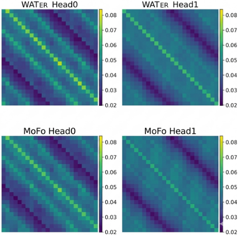
To examine the effectiveness of our proposed second-order difference maximization on token attention weights in our WATER, we present the visualizations on attention token weights of each self-attention head in Fig. 3. Comparing with MoFo, i.e. the backbone of our WATER, the token attention weights produced by our approach exhibit a clearer wave-like pattern, along with a clearer diagonal correlation structures. Moreover, the contrasts between higher and lower attention weights are enhanced to some extent. The higher weights of each token are more concentrated with its corresponding neighbors and meanwhile the lower weights are slightly suppressed. This indicate that our method can produce clearer and more structural attentions, making it less sensitive to possible noisy temporal patterns. Meanwhile, our WATER also mitigate the extreme-token phenomena in "Head1", further indicating that our WATER is capable of capturing more accurate temporal patterns to promote the forecasting performance.
Forecasting Visualization
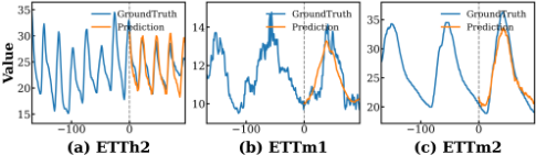
We present the forecasting visualizations on ETTh2, ETTm1 and ETTm2 in Fig. 4. We can find that our method can predict sequences which fit the ground-truth trends and key fluctuations well, and the predicted curves are smooth. This indicate that our method can effectively capture the temporal patterns to produce accurate and stable forecasting, making it practical in time series forecasting task.
Sensitivity on Scaling parameter λ
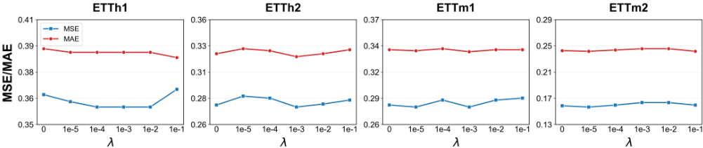
We examine the sensitivity of the scaling parameter λ, which controls the weight of the our proposed second-order difference maximization regularization term. We vary it over {1e - 5, 1e - 4, 1e - 3, 1e - 2, 1e - 1} on all 8 datasets and evaluate the forecasting performance. Results of 4 ETT datasets are presented in Fig. 5 and full results of 8 datasets are presented in Fig. 22 in Appendix. Overall speaking, WATER demonstrates low sensitivity to λ across all datasets, with both MSE and MAE remaining relatively stable over the range of values, indicating the robustness of our method. A slight performance degradation is observed when λ = 0 (i.e., the regularization term is disabled) on several datasets such as ETTh1 and Weather, indicating the effectiveness of the regularization in guiding the noise learning process. Furthermore, excessively large values (e.g., λ = 1e-1) occasionally lead to minor degradation, suggesting that an overly strong regularization may interfere with the dominant forecasting objective. In practice, we recommend setting λ ∈ {1e-4, 1e-3} for stable and consistent performance across diverse datasets.
Sensitivity on Historical Sequence Length L
We evaluate the sensitivity of our WATER to the the historical length by varying the it over {96, 336, 512} on prediction horizons {96, 192, 336, 720} and present the forecasting performance of datasets Weather, Solar, Electricity and Traffic in Fig. 23 in Appendix. Overall, we observe a consistent trend that performance improves as the historical length increases across most settings and datasets. In particular, longer input sequences generally lead to lower prediction errors, especially for longer forecasting horizons, indicating that the model benefits from richer temporal context. This suggests that WATER is able to effectively leverage extended historical information to capture more comprehensive and stable temporal dynamics.
Efficiency Analysis
We present computational efficiency comparisons on dataset Solar of forecasting horizon 96 in Table 3, where we report the amount of all learnable parameters requiring gradient descent (Param.), floating point operations (FLOPs), peak GPU memory usage (Peak GPU) and training time of one epoch (Epoch Time). We compare the methods under the same time series forecasting library TFB [Qiu et al., 2024] and same environment. All results of each model are under the optimal hyper-parameters for fair comparison. The results indicate that our method introduces a small additional computational cost compared to the baseline methods. While optimizing the noise injection parameter may lead to slower convergence, potentially requiring more training time. Overall, our method maintains competitive computational efficiency against the prevalent baseline TSF methods.
| Method | Param. (M) | FLOPs (B) | Peak GPU (MB) | Epoch Time (s) |
|---|---|---|---|---|
| Crossformer PatchTST Pathformer iTransformer PDF MoFo MoFo [our para] | 3.82↑1560.9% 2.62↑1039.1% 5.72↑2387.0% 0.51↑121.7% 5.82↑2430.4% 0.36↑56.5% 0.23- | 166.1↑1931.8% 644.9↑7788.7% 27.99↑242.4% 2.66↓67.5% 208.0↑2444.3% 11.69↑43.0% 8.175- | 10698↑435.2% 29726↑1387.0% 12754↑538.0% 788↓60.6% 5616↑180.9% 3458↑73.0% 1771↓11.4% | 101↑405.0% 215↑975.0% 614↑2970.0% 18↓10.0% 25↑25.0% 18↓10.0% 17↓15.0% |
| WATER (ours) | 0.23 | 8.175 | 1,999 | 20 |
6 Conclusion
In this paper, we focus on investigating the effect of perturbations to transformer-based TSF methods. Firstly, we conduct extensive preliminary studies to evaluate the stability of transformer-based TSF methods over various types of noises. We surprisingly find that applying noises at appropriate levels can effectively promote the forecasting performance and make the token attention weights wavy. Inspired by thie phenomena, we propose a novel TSF method WATER which adaptively perturbs the training data by Gaussian perturbations with zero mean and a learnable standard deviation to control the perturbation level. We optimize the standard deviation parameter by maximizing the second-order differences of token attention weights, which encourages each token to exhibit wave-like attention patterns with locally high curvature. Empirical studies on 8 benchmark datasets indicates that our WATER can outperform strong TSF baseline methods and induce attention weights in wave-like patterns.
Acknowledgments
We would like to acknowledge support for this project from the National Natural Science Foundation of China (No.62276113).
@inproceedings{ijcai2026p558,
  title     = {Perturbation Matters in Time Series Forecasting: A Wave-attention-aware Transformer Method},
  author    = {Wang, Yiming and Su, Yiqing and Li, Ximing and Li, Changchun and Wang, Bing},
  booktitle = {Proceedings of the Thirty-Fifth International Joint Conference on
               Artificial Intelligence, {IJCAI-26}},
  publisher = {International Joint Conferences on Artificial Intelligence Organization},
  editor    = {Diego Calvanese},
  pages     = {5012--5020},
  year      = {2026},
  month     = {8},
  note      = {Main Track},
  doi       = {10.24963/ijcai.2026/558},
  url       = {https://doi.org/10.24963/ijcai.2026/558},
}
TY - CPAPER TI - Perturbation Matters in Time Series Forecasting: A Wave-attention-aware Transformer Method AU - Wang, Yiming AU - Su, Yiqing AU - Li, Ximing AU - Li, Changchun AU - Wang, Bing T2 - Proceedings of the Thirty-Fifth International Joint Conference on Artificial Intelligence, IJCAI-26 PB - International Joint Conferences on Artificial Intelligence Organization PY - 2026 SP - 5012 EP - 5020 DO - 10.24963/ijcai.2026/558 UR - https://doi.org/10.24963/ijcai.2026/558 ER -Copied
Machine-readable versions of this paper, for tools and AI agents:





