Learning to Sparsify Stochastic Linear Bandits

1 Introduction

Online decision-making under uncertainty, particularly the multi-armed bandit (MAB) framework, has been a central area of research [Auer et al., 2002; Lattimore and Szepesvári, 2020]. Stochastic linear bandits model the reward at each decision step t as an inner product of an unknown parameter θ∗ (i.e., context vector) and the action vector xt plus noise [Abbasi-Yadkori et al., 2011], offering a simple yet general approach to model sequential decision-making in recommendation systems and adaptive control [Li et al., 2010; Chu et al., 2011]. A key consideration in linear bandits for real-world settings is sparsity, i.e., the context vector is sparse and only a small subset of its features influences the rewards [Agrawal and Goyal, 2013; Bastani et al., 2021]. Exploiting this sparsity, especially in high dimensions, can lead to more efficient algorithms and improved regret [AbbasiYadkori et al., 2012; Russo et al., 2018]. However, considering sparsity introduces an additional layer of complexity into the algorithm design and regret analysis [Oh et al., 2021; Hao et al., 2020; Dai et al., 2023].

*Corresponding author.

The full version of this paper that includes all the proofs can be found on arXiv as [Wang et al., 2026].

Linear Bandits with Sparse Context Vector. The earlier work [Abbasi-Yadkori et al., 2012] established a ˜O(√HdT) regret bound for sparse linear bandits when the sparsity pattern of the unknown context vector is known, where H is the number of nonzero entries in θ∗ ∈ Rd . Later, [Pacchiano et al., 2022] studied sparse linear bandits with unknown sparsity pattern and [Jin et al., 2024] proved a ˜O(√HdT) regret using a randomized model selection approach. The work of [Oh et al., 2021; Ichikawa et al., 2024] further studied the sparse contextual linear bandits setting. However, the aforementioned work assumed that the sparsity pattern of the context vector remains fixed and does not change over time.

Combinatorial Multi-Armed Bandits (CMAB). In the standard CMAB setting, a learner selects a subset of base arms (i.e., a super-arm) at each step, and the reward is given by a function of the individual reward of each arm [Chen et al., 2013; Chen et al., 2016]. For linear reward functions, an upper confidence bound method adapted from linear bandits has been proposed, which chooses a super-arm from the predefined set of base arms [Gai et al., 2012]. For nonlinear reward functions, the recent work [Fourati et al., 2024] proposes an online algorithm that achieves a (1 - 1/e)-regret bound of ˜O(T 2/3 ) for i.i.d. sampled monotone stochastic submodular reward functions, which leverages offline approximation algorithms as black-box oracles [Nie et al., 2023]. A multi-agent grouped CMAB problem has been studied in [Vannella et al., 2023a; Vannella et al., 2023b], which uses a mean field approximation approach and characterizes its statistical and computational trade-off.

Online Combinatorial Optimization. A broader area of work studies cases when the decision-maker first chooses an action that is a subset of a ground set at each step, and then a set function of the chosen action is revealed to return the corresponding reward [Streeter and Golovin, 2008; Wan et al., 2023]. Since the chosen action set often needs to satisfy certain combinatorial constraints (e.g., cardinality constraints), the problem is also termed online combinatorial optimization [Golovin et al., 2014]. A difficulty emerges when the offline version of the problem (i.e., when the set functions are known) is NP-hard, which necessitates the use of α-regret that compares the cumulative reward from an online algorithm against an approximately optimal reward with ratio α in hindsight [Streeter and Golovin, 2008]. The ratio α ∈ (0, 1) is set to be the approximation ratio of an offline algorithm [Das and Kempe, 2018].

Motivation. In the linear bandits with sparse context vector θ∗, the sparsity pattern of the context vector is a prescribed condition, i.e., when choosing the action vector xt, the learner cannot modify the sparsity of θ∗. Since the reward depends on the inner product between θ∗ and xt, the sparsity of θ∗ directly enforces the same sparsity pattern on xt. We now ask the following natural questions: What if the learner must simultaneously determine the sparsity pattern of the action vector xt and the non-zero entries of xt? Can we design algorithms for the learner to achieve meaningful regret? We refer to the problem as learning to sparsify stochastic linear bandits. Such a problem arises in many applications, e.g., recommendation systems and stock marketing.

Contributions. Since finding an optimal sparse action is NP-hard in general, we are faced with the following challenge: How to efficiently minimize cumulative regret when the action selection at each step constitutes a potentially NP-hard problem? We tackle this challenge by introducing a novel algorithmic framework for learning to sparsify stochastic linear bandits. We propose an adaptively phased exploration and exploitation algorithm that decouples parameter learning via Ordinary Least Squares (OLS) from the combinatorial action selection, and employs subroutines for efficient selection of sparse actions. Our key contributions are:

• We show that an optimal sparse action is tractable under a Euclidean ball action set X. We introduce a novel adaptive warm-up strategy with a data-driven stopping condition that does not rely on prior knowledge of the unknown parameters. Leveraging this adaptive strategy to recover the support of the optimal sparse action, we establish a ˜O(d√T) regret.
• When finding optimal sparse solutions becomes intractable for general action sets, we propose a combinatorial greedy algorithm as a subroutine to select a sparse action efficiently. Based on the geometry of the action set, we distinguish between two cases: i) For strongly convex action sets (e.g., an ellipsoid), we propose an algorithm that adaptively recovers the support of a greedy sparse action via the notion of greedy gap, and prove a ˜O(d√T) α-regret, relying on Lipschitz continuity of the optimal action map due to strongly convexity. ii) For general compact action sets (e.g., a hypercube), we show that a non-adaptive phased exploration and exploitation algorithm achieves a ˜O(dT 2/3 ) α-regret.
• Finally, we validate our theoretical results using comprehensive numerical experiments across action sets with different geometries, including a recommendation system instance.

Our regret results for Euclidean ball and strongly convex action sets readily match the regret lower bounds for linear bandits without sparsity [Lattimore and Szepesvári, 2020].

Notation. For a matrix P ∈ Rd×d , let P ⊤, tr(P), (P)ij be its transpose, trace, and element in i-th row and j-th column, respectively. Let λmin(A), λmax(A) be the minimum and maximum eigenvalues of a positive definite matrix A, respectively. Let Id be the d-dimensional identity matrix. Denote [n] ≜ {1, . . . , n} for n ≥ 1. For any x ∈ Rd and any S ⊆ [d], let x(S) ∈ Rd be such that supp(x) = S and (x(S))i = (x)i for all i ∈ [d], where (x)i denotes the i-th element of x and supp(x) ≜ {i ∈ [d] : (x)i ̸= 0}. Denote by ai:j the sequence ai, ai+1, . . . , aj. For y ∈ R, let |y| be its absolute value. For a finite set S, let |S| be its cardinality.

2 ProblemFormulation and Preliminaries

The stochastic linear bandit problem models a scenario of learning under uncertainty [Dani et al., 2007; Abbasi-Yadkori et al., 2011; Lattimore and Szepesvári, 2020]. Over T time steps, a decision-maker sequentially picks an action xt from a feasible action space Xt ⊂ Rd and receives a reward Yt ∈ R, which is a random variable with mean determined by the inner product of the action and an unknown parameter θ∗ ∈ Rd , i.e., E[Yt|xt] = θ⊤ ∗ xt. The challenge is to devise a policy that minimizes the cumulative regret RT , which quantifies the sum of performance gaps between the optimal action in hindsight and the chosen action at each step:

This basic model assumes that the reward Yt depends on the current action xt; however, in many cases, the external environment has requirements for the number of non-zero components of the action vector xt. For instance, i) the number of non-zero components of xt must be smaller than H for a deterministic H ∈ [d] (H is known to the decision maker); ii) some components of the action vector xt are not available (remaining 0 at time t). Specifically, letting St = supp(xt), at each time step t, the decision maker needs to select

We make the following standard assumption on X .

Assumption 1. The set X ⊂ Rd is closed and bounded.

Remark 1. The action set Xt can generally change over time as in the standard stochastic linear bandits setup, e.g. [Abbasi-Yadkori et al., 2011]. More discussions on this is provided in [Wang et al., 2026].

The reward Yt at any time t is then given by

where ηt is a random noise satisfying the following condition. Assumption 2. For any t ∈ [T], ηt is a random noise drawn from a conditionally σ-sub-Gaussian distribution with unknown variance proxy σ, i.e., E[ηt | x1:t(S1:t), η1:t-1] = 0, and E[exp(ληt) | x1:t(S1:t), η1:t-1] ≤ exp( λ2 σ2 2 ) ∀λ ∈ R.

An optimal solution in hindsight (i.e., when θ∗ is known) to the sparsifying linear bandits problem described above is given by solving

Finding an optimal action x⋆ (S⋆ ) involves solving an optimal subset selection problem, which is generally NP-hard [Das and Kempe, 2018; Ye et al., 2025]. This computational barrier typically makes it intractable for any polynomialtime algorithm to compete with the true optimum, necessitating a relaxed performance benchmark known as α-regret [Kalai and Vempala, 2005; Cesa-Bianchi and Lugosi, 2006; Streeter and Golovin, 2008], which is given by

When α = 1, α-RT in (5) reduces to RT in (1). The α-regret defined in (5) compares against an α-approximation of the optimal action, where α ∈ (0, 1] is the approximation ratio of an algorithm for the offline version of problem (4).

A Relevant Problem Formulation. A sparse online linear optimization problem has been studied in [Ye et al., 2025]. At each step t, the learner selects xt ∈ Rd and St ⊆ [d] with |St| ≤ H and receives a reward given by ft(xt, St) = θ⊤ t xt(St), where θt ∈ Rd is potentially generated by an adversary. However, there is no regret guarantee for the bandit setting. The online linear optimization framework for a single continuous action (without sparsity consideration) has been studied in [Bubeck et al., 2012], which achieves a ˜O(√dT)- regret. In contrast, we study the stochastic linear bandits setting whose reward is a random variable given by (3).

Roadmap. Our algorithm design and regret analysis in the subsequent sections hinge on the geometry of the action set X. We will split our approach into: (i) Euclidean Ball Action Sets (Section 3), where we show the optimal sparse action can be computed exactly and efficiently; (ii) General Strongly Convex Action Sets (Section 4), where we utilize a greedy approximation algorithm to select a sparse action; and (iii) Extensions to General Compact Sets (Section 5), where we address action sets lacking strong convexity.

A fundamental property required for our analysis is the variation of the optimal value function h(S; θ) with respect to the parameter θ. We present the following proposition to characterize this variation at two levels. First, for general compact action sets, the value function itself is Lipschitz continuous. Second, when the action set is further strongly convex, we obtain a stronger regularity: the gradient of the value function (i.e., the optimal action) also becomes Lipschitz continuous. The latter extends the Smooth Best Arm Response (SBAR) condition used in [Rusmevichientong and Tsitsiklis, 2010] (leveraging the duality properties of strongly convex sets [Polovinkin, 1996, Corollary 4]) to our sparse support framework. 1

Proposition 1 (Lipschitz Continuity). Consider a compact set X, and let LX = supx∈X ∥x∥2 . For any fixed support set S ⊆ [d], the value function h(S; θ) defined as h(S; θ) = supx∈X,supp(x)⊆S θ⊤x is convex and Lipschitz continuous with respect to θ, i.e., for any θ1, θ2 ∈ Rd ,

1 According to [Polovinkin, 1996, Definition 1], a set S ⊆ Rd is said to be strongly convex set of radius R > 0 if we can represent it as an intersection of closed balls of radius R.

Furthermore, if X is strongly convex, the gradient of the value function, given by ∇θh(S; θ) = x⋆ (S; θ) (the unique optimal action given S ⊆ [d]), is also Lipschitz continuous. That is, there exists a smoothness constant Lgrad > 0 (depending on the curvature of X) such that:

3 Euclidean Ball Action Sets

We first consider the scenario when X is an ℓ2-ball (Euclidean ball) with radius Lmax, which permits the efficient and exact computation of the optimal sparse action. Furthermore, one can show that LX = Lgrad = Lmax in Proposition 1. The following proposition formalizes the closed-form solution for the optimal sparse action for ℓ2-ball action set.

Proposition 2 (Optimal Sparse Action on ℓ2-Ball). Let X = {x ∈ Rd : ∥x∥2 ≤ Lmax}. For any parameter vector θ ∈ Rd , the optimal H-sparse action x⋆ for x⋆ ∈ argmaxx∈X,supp(x)⊆[d],|supp(x)|≤H θ⊤x is given by x⋆ = Lmax · θ(SH) ∥θ(SH)∥2 , where SH is the set of indices corresponding to the H largest absolute values of θ.

Hence, finding the best H-sparse action x⋆ (S⋆ ) for a given θ can be done in polynomial time by selecting the top H largest-magnitude components of θ. However, a critical challenge arises when the support set St changes dynamically, and the mapping from a parameter vector θ to its optimal sparse support S⋆ θ is discontinuous.

Key ideas. To establish the desired ˜O(d√T) regret, it is essential to ensure the proposed algorithm operates on the true optimal support S⋆ θ∗ (which is simply denoted as S⋆ subsequently). To this end, we propose an Adaptive Warm-up Strategy that does not require any prior knowledge of the true signal gap (i.e., the difference between the H-th largest and the (H + 1)-th largest in the absolute value of the elements in θ∗). Instead of fixing the exploration length a priori, our algorithm continuously monitors the empirical gap ∆′c of the estimated parameter ˆ θc (i.e., the aforementioned difference computed from ˆ θc). In Lemma 2, we will show that the above approach ensures Algorithm 1 transitions to the exploitation phase after identifying the true optimal support S⋆ .

3.1 APSEE Algorithm

We now present the Adaptively Phased Sparse Exploration and Exploitation (APSEE) algorithm (Algorithm 1). The algorithm operates in cycles indexed by c. The cycle index c initializes as 1 and increments by 1 after each cycle, allowing the algorithm to dynamically adapt time steps during each cycle until the total horizon T is reached. Each cycle begins with an Exploration Phase, playing a spanning set of exploration arms. Subsequently, Algorithm 1 updates the OLS estimate ˆ θc using accumulated data (line 8). To identify the true support S⋆ , the algorithm performs a Support Verification step (lines 9-15): it computes an anytime error bound εc, sorts the absolute values based on the estimated ˆ θc of the components {i′1 , . . . , i′d }, and calculates the empirical gap ∆′c . If the stopping condition ∆′c > 2εc is satisfied, the support Sest is locked (i.e., fixed). Finally, the algorithm enters the Exploitation Phase (lines 16-20), executing the best action on Sest for c steps. A key advantage of APSEE is to operate without requiring prior knowledge of the total time horizon T. To ensure that the OLS estimator utilized in the Exploration Phase is well-defined and possesses the necessary concentration properties for our theoretical analysis, we impose the following regularity condition on the exploration actions.

Assumption 3 (Exploration Actions). There exists a set of d actions {b1(S1), . . . , bd(Sd)} ⊂ X with |Sk| ≤ H for all k ∈ [d], such that B ≜ ∑dk=1 bk(Sk)bk(Sk)⊤ is invertible. Let λ0 = λmin(B) > 0. For instance, the set of basis vectors for Rd satisfies this assumption.

Remark 2. The existence of a spanning set of sparse exploration actions in Assumption 3 is a mild and standard one in the linear bandit literature. For example, a similar assumption is made for the analysis of the phased exploration strategy in [Rusmevichientong and Tsitsiklis, 2010, Assumption 1(b)].Finding such a spanning set is straightforward; for instance, the standard basis vectors satisfy the condition. Later in Section 6, we empirically show the consistent sub-linear regret across varying choices of basis actions (e.g., standard, Gaussian-random, and uniform-random bases) as long as the invertibility condition of B holds.

3.2 Adaptive Support Recovery

To start with, we establish the theoretical correctness of our adaptive support detection mechanism (lines 9-15 of Algorithm 1). Since this mechanism relies on the OLS estimator ˆ θc computed from exploration actions, we provide a highprobability anytime upper bound on the estimation error.

Lemma 1 (Anytime High-Probability Bound on OLS Error). Consider the OLS estimator ˆ θc (expressed as (8) in Algorithm 1). Let δ ∈ (0, 1) and h1 = 2σ2Tr(B) λ20 . With probability at least 1 - δ, for all cycles c ≥ 1 in Algorithm 1 simultaneously, the estimation error satisfies:

Building on this error bound of ˆ θc, we demonstrate that monitoring the empirical gap ∆′c = |(ˆ θc)i′H | - |(ˆ θc)i′H+1 | is sufficient to guarantee that the estimated support S⋆ c (with S⋆ c = Sest in line 14) matches the true support S⋆ .

Lemma 2 (Support Consistency for Euclidean Ball Action Sets). Consider any c ≥ 1. Suppose ∥∥∥ ˆ θc - θ∗∥∥∥2 ≤ εc. Let the sorted indices of θ∗ be {i⋆1 , . . . , i⋆d } such that |(θ∗)i⋆1 | ≥ · · · ≥ |(θ∗)i⋆d |, i.e., the true support is S⋆ = {i⋆1 , . . . , i⋆H }. Similarly, let the sorted indices of ˆ θc be {i′1 , . . . , i′d } with estimated support S⋆ c = {i′1 , . . . , i′H }. If the empirical gap satisfies ∆′c = |(ˆ θc)i′H | - |(ˆ θc)i′H+1 | > 2εc, then S⋆ c = S⋆ .

This result provides the theoretical foundation for the warm-up (pure exploration) phase of our algorithm. Once the condition ∆′c > 2εc is met, we can safely get into the next exploitation phase and incur low regret.

Algorithm 1 APSEE

Input: Dimension d, sparsity H, confidence parameter δ. Requires: Exploration set {b1(S1), . . . , bd(Sd)} from Assumption 3.

• 1: Initialize: B = d∑ k=1 bk(Sk)bk(Sk)⊤, c = 1, t = 1.
• 2: Flag: SupportFound = False, Sest = ∅.
• 3: for c = 1, 2, . . . do

- Exploration Phase (d steps) -

• 4: for k = 1, . . . , d do
• 5: Play action bk and observe reward Yt.
• 6: Set Yk(c) = Yt.
• 7: t ← t + 1.
• 8: Compute OLS estimate ˆ θc using all past data:

• 9: if SupportFound is False then
• 10: Compute error bound εc = √ h1 ln(2dc2 /δ) c .

15:

SupportFound ← True.

- Exploitation Phase (c steps) -

• 16: if SupportFound is True then
• 17: Compute the best action on support Sest: ac = arg maxx∈X ,supp(x)⊆Sest ˆ θ⊤ c x.

• 19: Play action ac and observe reward Yt.
• 20: t ← t + 1.
• 21: c ← c + 1.

3.3 Regret Analysis for Algorithm 1

Having established that Algorithm 1 correctly identifies the support S⋆ before entering the exploitation phase, we can now bound its cumulative regret defined in (5). Note that we have α = 1 in (5), due to Proposition 2.

Theorem 1 (Regret Bounds for APSEE). Suppose Assumptions 1-3 hold. Assume the unknown parameter θ∗ has a nonzero signal gap ∆min = |(θ∗)i⋆H | - |(θ∗)i⋆H+1 | > 0, where i∗H and i∗H+1 are described in Lemma 2. Let δ ∈ (0, 1). Then, with probability at least 1 - δ:

• If T > dC0, the cumulative regret satisfies

• If T ≤ dC0, the cumulative regret satisfies

Here, ˜O(·) hides logT factor and C0 = O(h1∆-2 min ) is the duration of the warm-up phase in Algorithm 1.

Our analysis reveals that even with the additional constraint of sparse actions, we achieve a ˜O(d√T) regret matching standard linear bandits (without sparsity) [Abbasi-Yadkori et al., 2011], which is known to be the best-achievable regret for standard linear bandits [Lattimore and Szepesvári, 2020]. Investigating the matching Ω(d√T) regret lower bound in our sparse linear bandit setting is left as future work.

4 General Strongly Convex Action Sets

We now consider broader class of action sets X that are strongly convex, including ellipsoids and ℓp-balls for p ∈ (1, 2], satisfying the strict positive curvature conditions [Polovinkin, 1996; Vial, 1982]. Unlike ℓ2-ball, an explicit closed-form solution for the sparse optimization problem is generally unavailable for these sets [Natarajan, 1995]. Thus, obtaining the exact optimal sparse action typically requires enumerating all possible support sets, incurring high computational cost. To address this challenge, we adopt the greedy algorithm [Nemhauser et al., 1978], an efficient heuristic for combinatorial optimization. While the greedy algorithm may not recover optimal solution, it guarantees an α-approximate one, where the approximation ratio α is determined by the submodularity ratio (defined later) of the objective function.

4.1 Adaptive Support Recovery via Greedy Gap and APSEE-G Algorithm

We introduce the Adaptively Phased Sparse Exploration and Exploitation with Greedy (APSEE-G) algorithm (Algorithm 2). To start with, define the maximum expected reward achievable on a fixed support set S ⊆ [d] with parameter θ as

For a general strongly convex set X, the function h(S; θ) is convex and Lipschitz continuous with respect to θ according to Proposition 1. Let SG and SG c be the support sets obtained by running the greedy algorithm on the true parameter θ∗ and the estimate ˆ θc (obtained as (8) in Algorithm 1), respectively. Specifically, running on any given parameter θ, the greedy algorithm constructs the support set iteratively: starting with an empty set G0 ← ∅, at each step k = 1, . . . ,H, it adds an element v ∈ [d] \Gk-1 to Gk-1 that maximizes the marginal gain ρk(v; θ) = h(Gk-1 ∪ {v}; θ) - h(Gk-1; θ).

Greedy Gap and Lipschitz Continuity

We analyze the consistency of the greedy algorithm by defining the gap at each step k ∈ {1, . . . ,H}. Let G∗k-1 be the set of size k - 1 selected by the greedy algorithm given θ∗. Then, the marginal gain of an element v is ρk(v; θ∗) = h(G∗k-1 ∪ {v}; θ∗) - h(G∗k-1 ; θ∗) for all v ∈ [d] \ G∗k-1 . Let g∗ k be the best element and vsecond k be the second-best element at step k, i.e., g∗ k = argmaxv∈[d]\G∗k-1 ρk(v; θ∗) and vsecond k = argmaxv′∈[d]\G∗k-1 ,v′ ̸=g∗ k ρk(v′ ; θ∗). We define: (i) Step-wise Greedy Gap: δk = ρk(g∗ k ; θ∗) - ρk(vsecond k ; θ∗); (ii) MinimumGreedy Gap: ∆min = min k=1,...,H δk. (13)

Algorithm 2 APSEE-G

Input: Dimension d, sparsity H, confidence parameter δ, ac-

tion set X . Requires: Exploration set {b1(S1), . . . , bd(Sd)}, Lipschitz constant LX . 1: Initialize: B = d∑ k=1 bk(Sk)bk(Sk)⊤, c = 1, t = 1. 2: Flag: SupportFound = False, Sest = ∅. 3: for c = 1, 2, . . . do - Exploration Phase (d steps) - 4: Run lines 3-10 of Algorithm 1. // Greedy Process (lines 5-13) 5: Let G0 = ∅ and ∆Greedy c =∞. 6: for k = 1, . . . ,H do 7: Compute candidate marginal gains: 8: ρk(v; ˆ θc) = h(Gk-1 ∪ {v}; ˆ θc) - h(Gk-1; ˆ θc), ∀v ∈ [d] \ Gk-1. 9: Find gk = argmaxv ρk(v; ˆ θc). 10: Find vsecond = argmaxv̸=gk ρk(v; ˆ θc). 11: Compute ˆ δk = ρk(gk; ˆ θc) - ρk(vsecond; ˆ θc). 12: Update gap: ∆Greedy c =min(∆Greedy c , ˆ δk). 13: Update set: Gk = Gk-1 ∪ {gk}. 14: if ∆Greedy c > 2LXεc then 15: Set Sest = GH. 16: SupportFound ← True. - Exploitation Phase (c steps) - 17: if SupportFound is True then 18: Compute optimal action on support Sest: ac = arg maxx∈X ,supp(x)⊆Sest ˆ θ⊤ c x. 19: for j = 1, . . . , c do 20: Play action ac and observe reward Yt. 21: t ← t + 1. 22: c ← c + 1.

Without loss of generality, we assume that ∆min > 0; otherwise, one can consider the third best element vthird k such that vthird k ̸= vsecond k and vthird k ̸= g∗ k . To relate the estimation error to the true support recovery, we again use the Lipschitz property (Proposition 1). Given that ∥∥∥ ˆ θc - θ∗∥∥∥2 ≤ εc, we have |h(S; ˆ θc)-h(S; θ∗)| ≤ LX εc, where LX = supx∈X ∥x∥2 in Proposition 1 and εc is defined in Lemma 1. Consequently, the error in estimating the marginal gain ρk(v; ·) (which is the difference of two h(·) values) is bounded by:

Stopping Condition and Consistency Lemma

To guarantee SG c = SG for some c ≥ 1, the idea is that the empirical gap ∆Greedy c (calculated in line 12 of Algorithm 2 using the estimate ˆ θc) must be large enough to overcome the estimation error of ˆ θc. Specifically, we need to distinguish the best element g∗ k from the second-best element vsecond k despite the estimation error in ˆ θc. Similar to the discussions in Section 3.2, we prove the following result.

Lemma 3 (Support Consistency for Strongly Convex Sets). Suppose ∥∥∥ ˆ θc - θ∗∥∥∥2 ≤ εc holds. Let ∆Greedy c be the minimum empirical marginal gain gap observed during the greedy algorithm execution on ˆ θc. If the stopping condition in line 14 holds: ∆Greedy c > 2LXεc, then the support set SG c obtained by running the greedy algorithm on ˆ θc is identical to the support set SG obtained by running the greedy algorithm on the true parameter θ∗.

4.2 Regret Analysis for Algorithm 2

We introduce the submodularity ratio for set functions, which plays a crucial role in proving the approximation ratio of greedy algorithms [Das and Kempe, 2018].

Definition 1. The submodularity ratio of a set function g : 2[n] → R≥0 is the largest γ ∈ R such that for all S, Ω ⊆ [n],

Recalling the α-regret defined in (5), we will let α = 1 - e-γ and derive the corresponding α-regret upper bound, where γ is the submodularity ratio of the set function h(S; θ) (with respect to S ⊆ [d]) defined in (12). We now show the following essential result that γ > 0, which implies that α > 0, i.e., the α-regret is not vacuous.

Proposition 3 (Submodularity Ratio for General (Strongly) Convex Sets). Let X be a convex compact set containing the origin. For any fixed parameter θ, consider the set function h(S; θ) = maxx∈X,supp(x)⊆S θ⊤x. The submodularity ratio γ of h(·; θ) is lower bounded by:

Moreover, γ > 0 when θ satisfies ∃x ∈ X , s.t. θ⊤x ̸= 0.

It is worth mentioning that when X is an ellipsoid X = {x ∈ Rd : x⊤Ax ≤ 1}, where A is positive definite and assumed without loss of generality that λmax(A) ≤ 1, the submodularity ratio γ of the set function h(·) in Proposition 3 satisfies that γ > λmin(A). More discussions on the ellipsoid case are deferred to [Wang et al., 2026]. Under the above guarantees and the condition that the greedy supports match (i.e., SG c = SG), we derive the regret upper bound for Algorithm2.

Theorem 2 (Regret bounds for APSEE-G). Suppose Assumptions 1-3 hold. Let Lmax = maxx∈X ∥x∥2 . Assume the true parameter θ∗ satisfies the Minimum Greedy Gap (13) condition with ∆min > 0. Let δ ∈ (0, 1). Then, with probability at least 1- δ:

• If T > dC0, the cumulative α-regret satisfies

• If T ≤ dC0, the cumulative α-regret satisfies

Here, ˜O(·) hides logT factor; C0 = O(h1∆-2 min ) is the warm-up phase length in Algorithm 2; α = 1 - e-γ , and γ is the submodularity ratio of h(·; θ∗) defined as (12).

5 General Compact Action Sets

When the action set X is a general compact set (e.g., a hypercube or a polytope), it does not necessarily possess the strong convexity property (curvature) as the Euclidean balls or ellipsoids. As discussed in Section 4, we use the submodularity ratio γ of the set function h(S; θ) = maxx∈X,supp(x)⊆S θ⊤x (with S ⊆ [d]) to parameterize the α-regret as α = 1 - e-γ . To ensure γ > 0 for general compact set X, we make the following assumption.

Assumption 4 (Convex Hull Regularity). Let X ⋆ = {x⋆ (S) : S ⊆ [d], |S| ≤ H}, where x⋆ (S) ∈ arg maxx∈X ,supp(x)⊆S θ⊤ ∗ x. Assume that conv(X ⋆ ) ⊆ X. 2

One can show that Assumption 4 directly holds for convex X . Under Assumption 4, we show in [Wang et al., 2026] that h(·; θ∗) possesses a strictly positive submodularity ratio γ > 0. We then prove the following regret bounds for a modified version of Algorithm 2.

Theorem 3 (Regret Bounds for General Compact Sets). Suppose Assumptions 1-4 hold. Run a modified version of Algorithm 2, which skips the support verification step (lines 14-17) and sets the exploitation length (line 19) to be ⌊√c⌋ for every cycle c = 1, 2, . . . . Let δ ∈ (0, 1). Then, with probability at least 1 - δ, the cumulative α-regret satisfies α-RT = ˜O (dT 2/3 ), where ˜O(·) hides logT factor, α = 1-e-γ , and γ is the submodularity ratio of h(·; θ∗) defined as (12).

6 Numerical Experiments

We empirically validate the theoretical performance and core mechanisms of our proposed algorithms. We focus our primary evaluation on the ellipsoid action set, which belongs to the strongly convex setting discussed in Section 4. We refer the readers to [Wang et al., 2026] for additional experiments on Euclidean balls, general compact sets, and a recommendation system application.

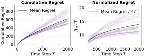
Regret Performance on Ellipsoid Action Sets. We fix the action dimension to d = 20 and the sparsity constraint to H = 5. The true parameter θ∗ is drawn uniformly from the hypercube [-1, 1]d . We simulate the environment for 2,000 time steps, where the noise ηt in the reward is i.i.d. Gaussian noise drawn from N(0, 0.52 ). The results are based on 20 independent trials. We construct an ellipsoid action set X = {x ∈ Rd : x⊤Ax ≤ 1}, where A is a randomly generated positive definite matrix with λmax(A) ≤ 1. We employ the APSEE-G algorithm (Algorithm 2) and validate the results established in Theorem 2. Figure 1 (Left) illustrates the cumulative α-regret of Algorithm 2. The scatter cloud highlights the variance across different runs, while the mean trajectory demonstrates a sub-linear growth, indicating that the algorithm successfully learns the optimal sparse action. To verify the regret bounds provided in Theorem 2, Figure 1 (Right) plots the α-regret normalized by √T . The curve of the mean normalized regret stabilizes and exhibits a slow, logarithmic growth trend, confirming the ˜O(√T) bound established in Theorem 2.

2 The convex hull of a set S, denoted conv(S), is the intersection of all convex sets containing S [Bertsekas, 2015].

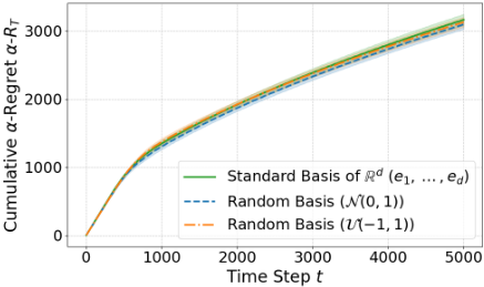
Impact of Basis Actions on Exploration. We examine the sensitivity of the APSEE-G algorithm (Algorithm 2) to the choice of basis actions utilized during the exploration phase. We conduct experiments using the following three distinct sets of basis actions under the same ellipsoid action set: (i) the standard basis vectors in Rd (consistent with the main evaluation), (ii) a random orthogonal basis generated from a standard Gaussian distribution, and (iii) a random orthogonal basis sampled from a uniform distribution. All these sets of basis actions satisfy the invertibility condition in Assumption 3. As illustrated in Figure 2, the cumulative α-regret trajectories of APSEE-G under these different basis sets are nearly indistinguishable, all exhibiting matching sub-linear growth rates. This empirical evidence corroborates the theoretical claims derived from Lemmas 2 and 3: provided that the chosen basis actions span the necessary space to satisfy Assumption 3, the exact distribution of the basis actions in the exploration phase has a negligible impact on the overall regret of the algorithm.

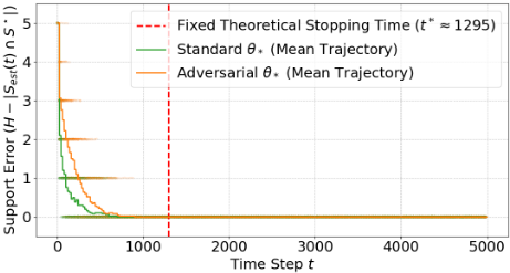
Empirical Verification of Support Recovery. While the recovery of the true support S⋆ is theoretically justified in Lemmas 2 and 3, we show that this guarantee holds in practical evaluations. To this end, we conduct additional experiments to track the real-time support recovery process of the APSEE algorithm (Algorithm 1) under two distinct configurations of the ground-truth parameter vector θ∗ ∈ R20 : a "standard" θ∗ (where the non-zero elements have more separated absolute values, making them easily identifiable) and an "adversarial" θ∗ (where the absolute values of the non-zero elements are nearly identical, making them highly difficult to distinguish). Both parameter vectors are constructed to share the exact same signal gap ∆min (defined as the absolute difference between the H-th and (H + 1)-th largest elements of θ∗). According to our theoretical proofs, sharing an identical ∆min ensures that the theoretical worst-case stopping time for the exploration phase, t∗ = O(1/∆2min ), is exactly the same for both cases. Figure 3 plots the evolution of the support recovery over time. For these two distinct cases, we conduct 50 trials each and plot scatter plots as well as average curves. The results clearly demonstrate that despite the differing difficulty landscapes of the standard and adversarial parameter vectors, the APSEE algorithm successfully identifies the true support S⋆ within the theoretical stopping time t∗ .

7 Conclusion

We formulated and analyzed the problem of learning to sparsify stochastic linear bandits with sparse action constraints. We proposed a novel algorithmic framework that effectively decouples parameter learning via OLS from combinatorial action selection. By leveraging an adaptive warm-up mechanism, we achieved ˜O(d√T ) regret for Euclidean and strongly convex action sets, and ˜O(dT 2/3 ) regret for compact sets. The regret upper bound ˜O(d√T) readily matches the minimax lower bound for standard linear stochastic bandits. Our results bridge the gap between high-dimensional linear bandits and online combinatorial optimization, opening future avenues for bandits or general RL problems with sparsity constraints on the chosen actions or policies.

Acknowledgments

This work was supported in part by the National Natural Science Foundation of China under Grants 62525603, U25A20469 and U24A20268; in part by the Key Research and Development Program of Hubei Province under Grants 2025BEB009. Please contact Lintao Ye (yelintao93@hust.edu.cn) for correspondence.