
Beyond Sequences: A Dynamic Hierarchical Heterogeneous Spatio-Temporal Graph for Irregular Multivariate Time Series Forecasting
Proceedings of the Thirty-Fifth International Joint Conference on Artificial Intelligence. Main Track. Pages 5146-5154.
https://doi.org/10.24963/ijcai.2026/573
Keywords
- Machine Learning: Time series and data streams
- Machine Learning: Sequence and graph learning
Abstract
Irregular Multivariate Time Series (IMTS) analysis is a challenging task as asynchronous irregular sampling disrupts intra-variable temporal consistency and cross-variable alignment. Most existing methods model multivariate correlations at either the variable or observation level in static ways. They suffer from correlation loss or cross-variable misalignment inevitably. In this paper, we propose a novel method DyH2-STGraph, Dynamic Hierarchical Heterogeneous Spatio-Temporal Graph, for IMTS forecasting. Within the graph, irregular observations are represented as nodes with spatio-temporal coordinates and observed values, connected with other neighbor observation nodes dynamically by spatio-temporal neighbor selection, while variables are treated as hyper nodes, connected with their constituent observation nodes as well as other variable nodes. The multivariate correlations are classified into the following three categories in specific manners: (1) Intra-variable coarse-to-fine correlations between variable nodes and their constituent observation nodes captured by hierarchical message propagation, (2) Inter-variable fine-grained correlations among neighboring observation nodes captured by spatio-temporal attention, and (3) Inter-variable coarse-grained correlations among variable nodes captured by attention. Extensive experiments on four benchmark datasets demonstrate that DyH2-STGraph significantly outperforms state-of-the-art methods while maintaining competitive efficiency.
- [Ansari et al., 2023] Abdul Fatir Ansari, Alvin Heng, Andre Lim, and Harold Soh. Neural continuous-discrete state space models for irregularly-sampled time series. In Pro- ceedings of the 40th International Conference on Machine Learning (ICML), volume 202 of Proceedings of Machine Learning Research, pages 926-951. PMLR, 2023.
- [Biloš et al., 2021] Marin Biloš, Johanna Sommer, Syama Sundar Rangapuram, Tim Januschowski, and Stephan Günnemann. Neural flows: Efficient alternative to neural odes. Advances in neural information processing systems, 34:21325-21337, 2021.
- [Cao et al., 2020] Defu Cao, Yujing Wang, Jianhui Duan, Chao Zhang, Xiaoping Zhu, Chang Huang, Yunhai Tong, Bixiong Xu, Jing Bai, Jie Tong, et al. Spectral temporal graph neural network for multivariate time-series forecast- ing. Advances in Neural Information Processing Systems, 33:17766-17778, 2020.
- [Che et al., 2018] Zhengping Che, Sanjay Purushotham, Kyunghyun Cho, David Sontag, and Yan Liu. Recurrent neural networks for multivariate time series with missing values. Scientific Reports, 8(1):6085, 2018.
- [Chen et al., 2018] Ricky TQ Chen, Yulia Rubanova, Jesse Bettencourt, and David K Duvenaud. Neural ordinary dif- ferential equations. Advances in neural information pro- cessing systems, 31, 2018.
- [Chen et al., 2021] Yuzhou Chen, Ignacio Segovia, and Yu- lia R. Gel. Z-gcnets: Time zigzags at graph convolutional networks for time series forecasting. In International Con- ference on Machine Learning, PMLR, pages 1684-1694, 2021.
- [Chowdhury et al., 2023] Rakshith R Chowdhury, Jialu Li, Xiyuan Zhang, Di Hong, Rajesh K Gupta, and Jingbo Shang. Primenet: Pre-training for irregular multivariate time series. In Proceedings of the AAAI Conference on Ar- tificial Intelligence, volume 37, pages 7184-7192, 2023.
- [Cini et al., 2021] Andrea Cini, Ivan Marisca, and Cesare Alippi. Filling the g ap s: Multivariate time series im- putation by graph neural networks. In International Con- ference on Learning Representations, 2021.
- [De Brouwer et al., 2019] Edward De Brouwer, Jaak Simm, Adam Arany, and Yves Moreau. Gru-ode-bayes: Con- tinuous modeling of sporadically-observed time series. In Advances in Neural Information Processing Systems (NeurIPS), pages 7377-7388, 2019.
- [De Gooijer and Hyndman, 2006] Jan G. De Gooijer and Rob J. Hyndman. 25 years of time series forecasting. In- ternational Journal of Forecasting, 22(3):443-473, 2006.
- [Han et al., 2024] Jialin Han, Wenxuan Zhang, Haotian Liu, Tiantian Tao, Ning Tan, and Hui Xiong. Bigst: Linear complexity spatio-temporal graph neural network for traf- fic forecasting on large-scale road networks. Proceedings of the VLDB Endowment, 17(5):1081-1090, 2024.
- [Horn et al., 2020] M. Horn, M. Moor, C. Bock, B. Rieck, and K. M. Borgwardt. Set functions for time series. In Proceedings of the 37th International Conference on Ma- chine Learning (ICML), volume 119, pages 4353-4363, 2020.
- [Kidger et al., 2020] Patrick Kidger, James Morrill, James Foster, and Terry Lyons. Neural controlled differential equations for irregular time series. Advances in neural in- formation processing systems, 33:6696-6707, 2020.
- [Li and Marlin, 2020] Steven Cheng-Xian Li and Ben- jamin M. Marlin. Learning from irregularly-sampled time series: A missing data perspective. In Proceedings of the 37th International Conference on Machine Learning (ICML), volume 119 of Proceedings of Machine Learning Research, pages 5937-5946. PMLR, 2020.
- [Li et al., 2025] Boyuan Li, Yicheng Luo, Zhen Liu, Junhao Zheng, Jianming Lv, and Qianli Ma. Hyperimts: Hyper- graph neural network for irregular multivariate time series forecasting. In Proceedings of the 42nd International Con- ference on Machine Learning (ICML), 2025.
- [Liu et al., 2024] Yong Liu, Tengge Hu, Haoran Zhang, Haixu Wu, Shiyu Wang, Lintao Ma, and Mingsheng Long. itransformer: Inverted transformers are effective for time series forecasting. In The Twelfth International Confer- ence on Learning Representations, 2024.
- [Liu et al., 2026a] Xvyuan Liu, Xiangfei Qiu, Hanyin Cheng, Xingjian Wu, Chenjuan Guo, Bin Yang, and Jilin Hu. Astgi: Adaptive spatio-temporal graph interactions for irregular multivariate time series forecasting, 2026.
- [Liu et al., 2026b] Xvyuan Liu, Xiangfei Qiu, Xingjian Wu, Zhengyu Li, Chenjuan Guo, Jilin Hu, and Bin Yang. Re- thinking irregular time series forecasting: A simple yet ef- fective baseline. In Proceedings of the 40th AAAI Confer- ence on Artificial Intelligence, 2026. Oral Presentation.
- [Luo et al., 2025] Yicheng Luo, Bowen Zhang, Zhen Liu, and Qianli Ma. Hi-patch: Hierarchical patch gnn for irreg- ular multivariate time series. In Proceedings of the 42nd International Conference on Machine Learning (ICML), 2025.
- [Mercatali et al., 2024] G. Mercatali, A. Freitas, and J. Chen. Graph neural flows for unveiling systemic interactions among irregularly sampled time series. In Advances in Neural Information Processing Systems (NeurIPS), 2024.
- [Nie et al., 2023] Yuqi Nie, Nam H. Nguyen, Phanwadee Sinthong, and Jayant Kalagnanam. A time series is worth 64 words: Long-term forecasting with transformers. In International Conference on Learning Representations (ICLR), 2023.
- [Satorras et al., 2022] Victor Garcia Satorras, Syama Sundar Rangapuram, and Tim Januschowski. Multivariate time series forecasting with latent graph inference, 2022.
- [Schirmer et al., 2022] M. Schirmer, M. Eltayeb, S. Less- mann, and M. Rudolph. Modeling irregular time series with continuous recurrent units. In Proceedings of the 39th International Conference on Machine Learning (ICML), volume 162, pages 19388-19405, 2022.
- [Shukla and Marlin, 2020] Satya Narayan Shukla and Ben- jamin M. Marlin. A survey on principles, models and methods for learning from irregularly sampled time series: From discretization to attention and invariance. CoRR, abs/2012.00168, 2020.
- [Shukla and Marlin, 2021] Satya Narayan Shukla and Ben- jamin Marlin. Multi-time attention networks for irregu- larly sampled time series. In International Conference on Learning Representations, 2021.
- [Vaswani et al., 2017] Ashish Vaswani, Noam Shazeer, Niki Parmar, Jakob Uszkoreit, Llion Jones, Aidan N Gomez, Ł ukasz Kaiser, and Illia Polosukhin. Attention is all you need. In I. Guyon, U. Von Luxburg, S. Bengio, H. Wal- lach, R. Fergus, S. Vishwanathan, and R. Garnett, editors, Advances in Neural Information Processing Systems, vol- ume 30.
- Curran Associates, Inc., 2017.
- [Vio et al., 2013] Roberto Vio, Mara Daz-Trigo, and Paola Andreani. Irregular time series in astronomy and the use of the lomb-scargle periodogram. Astronomy and Comput- ing, 1:5-16, 2013.
- [Wen et al., 2023] Haomin Wen, Youfang Lin, Yutong Xia, Huaiyu Wan, Qingsong Wen, Roger Zimmermann, and Yuxuan Liang. Diffstg: Probabilistic spatio-temporal graph forecasting with denoising diffusion models. In Pro- ceedings of the 31st ACM International Conference on Ad- vances in Geographic Information Systems, pages 1-12. ACM, 2023.
- [Wu et al., 2020] Zonghan Wu, Shirui Pan, Guodong Long, Jing Jiang, Xiaojun Chang, and Chengqi Zhang. Con- necting the dots: Multivariate time series forecasting with graph neural networks. In Proceedings of the 26th ACM SIGKDD International Conference on Knowledge Discov- ery & Data Mining, pages 753-763, 2020.
- [Yalavarthi et al., 2024] Vijaya Krishna Yalavarthi, Kiran Madhusudhanan, Randolf Scholz, Nourhan Ahmed, Jo- hannes Burchert, Shayan Jawed, Stefan Born, and Lars Schmidt-Thieme. Grafiti: Graphs for forecasting irreg- ularly sampled time series. In Proceedings of the AAAI Conference on Artificial Intelligence, volume 38, pages 16255-16263, 2024.
- [Yao et al., 2018] Zhenjie Yao, Jie Bi, and Yixin Chen. Ap- plying deep learning to individual and community health monitoring data: A survey. International Journal of Au- tomation and Computing, 15(6):643-655, 2018.
- [Yi et al., 2023] Kun Yi, Qi Zhang, Wei Fan, Hui He, Liang Hu, Peng Wang, Ning An, Longbing Cao, and Zhendong Niu. Fouriergnn: Rethinking multivariate time series fore- casting from a pure graph perspective. In Advances in Neural Information Processing Systems, volume 36, pages 15147-15159, 2023.
- [Zeng et al., 2022] Ailing Zeng, Mu-Hwa Chen, L. Zhang, and Qiang Xu. Are transformers effective for time se- ries forecasting? In AAAI Conference on Artificial Intelli- gence, 2022.
- [Zhang et al., 2022] Xiang Zhang, Marko Zeman, Theodoros Tsiligkaridis, and Marinka Zitnik. Graph- guided network for irregularly sampled multivariate time series. In International Conference on Learning Representations (ICLR), 2022.
- [Zhang et al., 2023] Jiawen Zhang, Shun Zheng, Wei Cao, Jiang Bian, and Jia Li. Warpformer: A multi-scale model- ing approach for irregular clinical time series. In Proceed- ings of the 29th ACM SIGKDD Conference on Knowledge Discovery and Data Mining (SIGKDD), pages 3273-3285, 2023.
- [Zhang et al., 2024] Weijia Zhang, Chenlong Yin, Hao Liu, Xiaofang Zhou, and Hui Xiong. Irregular multivariate time series forecasting: A transformable patching graph neural networks approach. In Proceedings of the 41st Interna- tional Conference on Machine Learning (ICML), 2024.
References were extracted automatically from the PDF and may contain errors.
Full text extracted automatically from the PDF; figures, tables and equations may differ. The PDF is the version of record.
1 Introduction
Irregular Multivariate Time Series (IMTS) forecasting is a critical task in various domains, including clinical medicine, financial analysis, and industrial monitoring [Yao et al., 2018; Vio et al., 2013; Shukla and Marlin, 2020; De Brouwer et al., 2019]. Unlike regularly sampled time series, IMTS are characterized by asynchronous observation timestamps across variables, heterogeneous sampling frequencies, and pervasive missing values. Despite recent advancements, accurately capturing the latent dependencies within such irregularlysampled data remains a significant challenge.
† Corresponding author
To address the inherent irregularity, conventional methods predominantly rely on alignment-based preprocessing, such as interpolation, resampling, or patching [De Gooijer and Hyndman, 2006; Zeng et al., 2022]. However, these manual imputation or resampling strategies introduces non-trivial inductive biases, which can distort the underlying data distribution [Ansari et al., 2023]. While patching avoids explicit point-wise alignment, it inevitably leads to boundary effects and data truncation. These issues obscure high-frequency dynamics and, in scenarios of extreme sparsity, result in the irretrievable loss of inherent irregular patterns [Nie et al., 2023; Zhang et al., 2023]. Standard sequence-modeling architectures, such as Recurrent Neural Networks (RNNs) and Transformers, exhibit limitations when applied to IMTS [Li and Marlin, 2020]. RNNs typically assume uniform time steps between transitions, failing to account for temporal decay or state evolution during variable intervals. Similarly, standard Transformers utilize discrete positional encodings that are unsuitable for representing the continuous nature of time [Vaswani et al., 2017].
While graph-based representations have emerged as a promising alternative, they often encounter a structural tradeoff between modeling precision and computational complexity [Yalavarthi et al., 2024; Li et al., 2025]. Modeling IMTS as a global fully-connected graph incurs prohibitive computational costs and risks diluting of salient information by global noise [Luo et al., 2025]. Conversely, localized graph models, while more efficient, suffer from restricted receptive fields and a lack of global contextual awareness [Liu et al., 2026a]. Consequently, neither approach effectively captures the multi-scale dependencies required for robust IMTS analysis. Although some advanced models adopt dimensional decoupling strategy to process temporal and variable dependencies separately, this approach restricts correlations to axis-parallel directions [Liu et al., 2024]. Such a design ignores the intrinsic spatio-temporal coupling of local dynamics, forcing the model to rely on multiple stacked layers to indirectly reconstruct cross-variable interactions. This architectural constraint significantly reduces sensitivity to finegrained, instantaneous dependencies.
To address these limitations, we propose the Dynamic Hierarchical Heterogeneous Spatio-Temporal Graph (DyH2STGraph). Instead of constraining irregular observations to a rigid grid, DyH2-STGraph adopts a graph-centric perspective, where observations are represented as nodes with spatiotemporal coordinates. Meanwhile, to reconcile the trade-off between local precision and global context, our framework introduces a variable-level hypernode. These two types of nodes are connected through three categories of edges, enabling a three-fold correlation decomposition: (1) Hierarchical edges bridge observation nodes with their corresponding variable hypernodes, facilitating intra-variable coarse-to-fine correlation capture. (2) Spatio-temporal edges are dynamically established between neighboring observation nodes via a neighbor selection mechanism, facilitating inter-variable fine-grained correlation capture. (3) Horizontal edges connect all hypernodes, enabling inter-variable coarse-grained correlation capture. By leveraging these heterogeneous nodes and edges, DyH2-STGraph effectively captures the multigrained, non-stationary correlations inherent in IMTS. Our major contributions are summarized as follows:
- We introduce a dynamic hierarchical heterogeneous spatio-temporal graph paradigm specifically tailored for IMTS. This approach naturally accommodates asynchronous observations across variables, effectively bypassing the need for traditional alignment or imputation.
- We propose a comprehensive mechanism to disentangle IMTS correlations into three levels: intra-variable hierarchical, inter-variable fine-grained, and inter-variable coarse-grained correlations. Facilitated by three distinct categories of edges of the graph, this decomposition enables more robust representation learning.
- We conducted extensive experiments on four public benchmark datasets. The results demonstrate that DyH2-STGraph consistently outperforms state-of-theart baselines. In-depth analyses further validate the effectiveness of each proposed component in modeling multivariate correlations.
2 RelatedWork
2.1 Irregular Multivariate Time Series Modeling
IMTS modeling faces unique challenges from asynchronous sampling and heterogeneous temporal gaps. Existing approaches fall into four paradigms: (1) Continuous-time Dynamics Models: Neural ODEs and flows-based frameworks parameterize latent dynamics as continuous functions, naturally handling arbitrary temporal gaps [Chen et al., 2018; Kidger et al., 2020; Biloˇs et al., 2021; Mercatali et al., 2024; Schirmer et al., 2022]. However, they incur substantial computational overhead and may struggle with high-dimensional dependencies. (2) Standard MTS Adaptation Models: These methods adapt conventional architectures through time-aware mechanisms: RNN-based methods use trainable decay or gating [Che et al., 2018], attention-based approaches map observations to reference points [Shukla and Marlin, 2021], and Transformers employ discrete encodings or warping [Zhang et al., 2023]. Despite effectiveness, their reliance on fixedstep transitions, and require alignment operations that may distort intrinsic temporal patterns. (3) Set-based Models: These methods treat observations as permutation-invariant sets, bypassing temporal alignment [Horn et al., 2020]. While efficient, they sacrifice precise temporal ordering, limiting their capacity for high-frequency dynamics. (4) Graph-based Models: Graph provide a flexible paradigm for modeling complex relational structures in IMTS [Wu et al., 2020; Han et al., 2024]. They typically represent variables as nodes and their dependencies as edges, using sparse representations to handle IMTS samples without padding. While showing promise for IMTS modeling, they still suffer from architectures restricts. We discussed in detail in Section 2.2.
2.2 Using Graphs for IMTS
Graph are increasingly popular in IMTS analysis[Li et al., 2025; Yi et al., 2023; Wen et al., 2023; Cini et al., 2021]. Early GNN-based approaches required a predefined adjacency matrix to establish relationships between variables [Wu et al., 2020]. However, these methods often rely on fixed topologies that cannot adapt to transient, non-stationary dependencies. To address this challenge, recent models have integrated graph learning components to dynamically capture dependencies between variables [Cao et al., 2020; Chen et al., 2021]. Existing graph-based models primarily focus on learning correlations at either the variable level [Zhang et al., 2022] or the node level [Yalavarthi et al., 2024]. Nevertheless, they often fail to fully exploit complex graph structures, leading to inevitable correlation loss. Furthermore, while some recent approaches utilize hypergraphs or bipartite graphs to capture correlations flexibly [Li et al., 2025; Satorras et al., 2022; Yalavarthi et al., 2024], they typically process temporal and variable dependencies separately, which restricts correlations to axis-aligned directions and results in suboptimal performance. Some methods initialize data-driven contexts to capture the intrinsically coupled nature of local spatio-temporal dynamics [Liu et al., 2026a]. However, their graph structures often remain static during the message-passing process, limiting their capacity to capture evolving correlations.
3 ProblemDefinition
We consider an IMTS dataset D. With a total of T timestamps and M variables, each IMTS sample S ∈ D can be denoted as a collection of observation triplets: S = {(ti, vi, xi) | i = 1, . . . ,N}, where ti ∈ {1, . . . , T}, vi ∈ {1, . . . ,M} , xi ∈ R represent the timestamp, variable indicator, observed value respectively, and N represent the total number of observations in the sample S. For the IMTS forecasting task, given a split timestamp tS, an IMTS sample is divided into a lookback window X = {(ti, vi, xi) ∈ S | ti ≤ tS} and a forecast window Y = {(ti, vi, xi) ∈ S | ti > tS}. The forecast query qi ∈ Q is derived by combining (ti, vi) of the i-th observation triplet within the forecast window. We aim to learn a forecasting model F(·), such that given the lookback window X and forecast query Q as input, it accurately predicts the corresponding observed values Z:
of forecast target initialized to 0. The value embedding of node i is given by:
where FFobs is a learnable projection, and ⊕ denotes the concatenation operation. Imask ∈ {0, 1} indicates whether node i is a padding node.
Finally, the representation of node i is (pi, h(0) i ), with the spatio-temporal coordinate defined as:
Hypernode Representation. We define a set of learnable global parameters Ws ∈ RM×dmodel to initialize the hypernodes corresponding to M variables. The initial state of the v-th variable hypernode is given by:
4.2 Intra-variable Coarse-to-fine Correlation Capturer
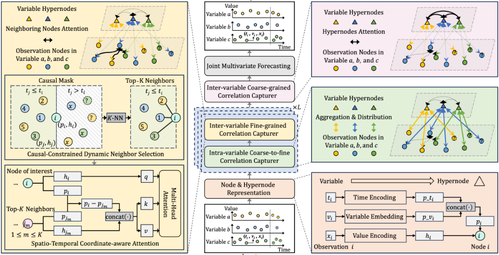
We propose a bidirectional hierarchical message propagation to capture intra-variable coarse-to-fine correlations between variable hypernodes and their constituent observation nodes, that is, Bottom-up Coarse-grained Aggregation first, and then Top-down Fine-grained Refinement.
Bottom-up Coarse-grained Aggregation. In this phase, observation nodes associated with the same variable are aggregated to obtain a representative hypernode embedding.
4 Methodology
Figure 1 shows the DyH2-STGraph framework. All modules are introduced in the following subsections in detail.
4.1 Node &Hypernode Representation
For each IMTS sample, irregular observations are represented as nodes with spatio-temporal coordinates and observed values, while variables are treated as hyper nodes. The two types of nodes can be represented as follows.
Observation Node Representation. Each observation node i denoted by (ti, vi, xi) is represented by:
(1) Temporal Embeddings, which is used to capture temporal distances in a continuous space by projecting the normalized timestamp ti:
(2) Spatial Embeddings, which is used to distinguish nodes across different variables by mapping the variable index vi:
(3) Value Embeddings, which is used to encode the node's feature. To distinguish between known observations and forecast targets, a binary indicator mi ∈ {0, 1} is concatenated with the numerical value xi before projection, with the value The membership is strictly governed by the variable incidence matrix I ∈ {0, 1}M×N , where Iv,i = 1 indicates that node i belongs to variable v (either as an observation or a forecast target). Notably, we employ a causal mask M ∈ {0, 1}N at the first layer to ensure that each variable hypernode aggregates only historical observation nodes initially, where Mi = 1 denotes that node i is an observation, and Mi = 0 denotes that node i is a forecast target. The representation of hypernode v is updated by:
This step transforms discrete, irregular nodes into coarsegrained hypernodes representing the overall semantic evolution of the variable.
Top-down Fine-grained Refinement. After aggregation, hypernode representations are redistributed to their constituent observation nodes. The representation of observation node i is refined by:
where svi denotes the hypernode for node i, ⊕ denotes concatenation, and FC denotes a linear fusion layer.
4.3 Inter-variable Fine-grained Correlation Capturer
We first introduce a Dynamic Neighbor Selection mechanism to determine which observation nodes across variables should be connected, and then employ Spatio-Temporal Coordinateaware Attention to encode fine-grained correlations among observation nodes across variables.
Causal-Constrained Dynamic Neighbor Selection. For each observation node, the dynamic neighbor selection mechanism only adaptively selects the most relevant K neighbors from all observation nodes to connect it. The distance between nodes is measured by a hybrid metric based on the static spatio-temporal coordinates p and dynamic latent states h. At layer l, the distance D(l) ij between node i and node j is defined as:D(l) ij = ˆ d(pi, pj) +ω(l) · ˆ d(h(l) i , h(l) j ), (10)
where ˆ d(·, ·) denotes the squared Euclidean distance, and ω(l) denotes the balancing weight which is defined as a linearly increasing function of network depth: ω(l) = λ×l, where λ is a hyperparameter. This design reflects the increasing discriminability of latent representations at greater network depths. Subsequently, we utilize a causal mask to prevent information leakage from future time steps, along with a padding mask to filter out padding nodes. The final distance matrix is given by:
Based on the distance matrix, we obtain a set of K neighbors N (l) i closest to each observation node i.
Spatio-Temporal Coordinate-aware Attention. For each observation node i, the Spatio-Temporal Coordinate-aware Attention mechanism is used to aggregate messages within the neighbors N (l) i .
Specifically, we employ the multi-head attention to model the spatio-temporal correlation between node i and its neighbor j based on the relative distance prel = pi - pj. The Query, Key, and Value representations are formulated as:
And the node representation is updated by:
4.4 Inter-variable Coarse-grained Correlation Capturer
After the iterations of the Intra-variable Coarse-to-fine and Inter-variable Fine-grained Correlation Capturers, we employ a self-attention mechanism to capture inter-variable coarsegrained correlation among variable hypernodes, defined as:
where s(L) ∈ RM×dmodel represents the hidden states of the M variable hypernodes output by the Inter-variable Finegrained Correlation Capturer after L layers of processing.
4.5 Joint Multivariate Forecasting
In the final stage, we employ a joint decoder for multivariate forecasting. For target node i ∈ Y, its final representation h(L) i and the final representation of its associated hypernode svi are fused together to predict its value ˆ yi:
where FCout denotes a linear projection layer. The model is trained by minimizing the Mean Squared Error (MSE) between the predicted values ˆ Z and the corresponding ground truth Z for the forecast queries.
| Dataset | PhysioNet'12 | MIMIC-III | HumanActivity | USHCN | ||||
|---|---|---|---|---|---|---|---|---|
| Metric | MSE | MAE | MSE | MAE | MSE | MAE | MSE | MAE |
| PrimeNet | 0.803±0.000 | 0.688±0.000 | 0.875±0.000 | 0.646±0.000 | 4.372±0.006 | 1.728±0.001 | 0.494±0.002 | 0.496±0.002 |
| SeFT | 0.781±0.002 | 0.679±0.002 | 0.899±0.001 | 0.649±0.002 | 1.410±0.013 | 0.990±0.005 | 0.335±0.004 | 0.408±0.013 |
| GNeuralFlow | 0.788±0.141 | 0.660±0.054 | 0.880±0.040 | 0.631±0.018 | 0.411±0.328 | 0.461±0.155 | 0.223±0.055 | 0.331±0.051 |
| mTAN | 0.388±0.006 | 0.433±0.004 | 0.946±0.136 | 0.674±0.053 | 0.096±0.006 | 0.223±0.010 | 0.666±0.153 | 0.523±0.068 |
| CRU | 0.631±0.005 | 0.585±0.004 | 0.728±0.008 | 0.575±0.004 | 0.139±0.012 | 0.262±0.013 | 0.214±0.028 | 0.319±0.027 |
| NeuralFlows | 0.408±0.007 | 0.449±0.006 | 0.634±0.021 | 0.531±0.009 | 0.176±0.014 | 0.317±0.015 | 0.209±0.042 | 0.316±0.030 |
| GRU D | 0.349±0.002 | 0.405±0.001 | 0.492±0.022 | 0.453±0.009 | 0.174±0.045 | 0.312±0.037 | 0.213±0.058 | 0.308±0.039 |
| Raindrop | 0.349±0.003 | 0.406±0.003 | 0.583±0.191 | 0.496±0.093 | 0.089±0.009 | 0.209±0.012 | 0.209±0.044 | 0.288±0.015 |
| Hi-Patch | 0.307±0.003 | 0.366±0.002 | 0.453±0.008 | 0.411±0.005 | 0.049±0.001 | 0.128±0.002 | 0.189±0.023 | 0.275±0.034 |
| tPatchGNN | 0.306±0.003 | 0.364±0.001 | 0.447±0.013 | 0.406±0.009 | 0.045±0.002 | 0.125±0.003 | 0.182±0.073 | 0.299±0.070 |
| Warpformer | 0.300±0.006 | 0.362±0.009 | 0.424±0.007 | 0.393±0.006 | 0.046±0.001 | 0.125±0.003 | 0.191±0.105 | 0.296±0.102 |
| APN | 0.308±0.002 | 0.364±0.003 | 0.433±0.004 | 0.402±0.002 | 0.041±0.013 | 0.116±0.006 | 0.163±0.022 | 0.263±0.032 |
| HyperIMTS | 0.294±0.002 | 0.356±0.002 | 0.363±0.002 | 0.365±0.003 | 0.047±0.003 | 0.132±0.007 | 0.185±0.016 | 0.280±0.014 |
| GraFITi | 0.300±0.003 | 0.359±0.006 | 0.377±0.002 | 0.373±0.003 | 0.044±0.001 | 0.124±0.002 | 0.174±0.018 | 0.272±0.016 |
| ASTGI | 0.297±0.004 | 0.357±0.003 | 0.408±0.015 | 0.392±0.011 | 0.041±0.001 | 0.118±0.001 | 0.159±0.009 | 0.261±0.019 |
| Ours | 0.290±0.001 | 0.352±0.001 | 0.350±0.003 | 0.355±0.004 | 0.041±0.001 | 0.117±0.004 | 0.155±0.012 | 0.254±0.019 |
5 Experiment
5.1 Experimental Setup
Datasets. We conduct experiments on four widely-used public IMTS datasets from various domains, including healthcare, biomechanics, and climate science. The PhysioNet'12 dataset provides clinical time series from the first 48 hours of ICU stays, which is rounded for 1 hour. MIMIC-III is also a clinical database collected from ICU patients during the first 48 hours of admission, which is rounded for 30 minutes. The HumanActivity dataset consists of biomechanics data with 3D positional variables captured from subjects performing various activities, which is rounded for 1 millisecond. USHCN includes climate data over 150 years collected by meteorological stations scattered over the United States, and we focus on a subset of 4 years between 1996 and 2000. To ensure fairness and comparability of the results, all datasets are preprocessed by strictly following the standard procedures established in prior state-of-the-art works [Li et al., 2025; Yalavarthi et al., 2024]. In line with established practices, all datasets are partitioned into training, validation, and test sets using a standard 80%, 10%, and 10% ratio, respectively. Training and validation sets are shuffled, while test sets are not.
Baselines. To evaluate the performance of DyH2-STGraph, we selected a total of fifteen state-of-the-art models designed for irregular time series as baselines. These include: (1) RNN and ODE-based methods, including GRU-D [Che et al., 2018], CRU [Schirmer et al., 2022], NeuralFlows [Biloˇs et al., 2021] and GNeuralFlow [Mercatali et al., 2024], (2) Set-based and Kernel-attention methods, including mTAN
[Shukla and Marlin, 2021] and SeFT [Horn et al., 2020], (3) Patch-based methods, including tPatchGNN [Zhang et al., 2024], Hi-Patch [Luo et al., 2025] and APN [Liu et al., 2026b], (4) Warping and hybrid Transformer methods, including Warpformer [Zhang et al., 2023], (5) Graph-based methods, including Raindrop [Zhang et al., 2022], PrimeNet [Chowdhury et al., 2023], GraFITi [Yalavarthi et al., 2024], ASTGI [Liu et al., 2026a] and HyperIMTS [Li et al., 2025].
ImplementationDetails. All models are trained on a Linux server with PyTorch version 2.6.0+cu124 using four NVIDIA Tesla V100-DGXS-32GB GPUs. All experiments run with a maximum epoch number of 300 and early stopping patience of 10 epochs. All models are trained using the Mean Squared Error (MSE) as the loss function and optimized with the Adam optimizer. The learning rate Ln for the n-th epoch is kept unchanged when n ≤ 3, and adjusted according to Ln = L0 ×0.8n-3 when n > 3. To ensure a fair comparison, we primarily adopted the hyperparameter settings reported in the original papers for the baseline models. To mitigate randomness, each experiment is run independently with five different random seeds from 2024 to 2028, and we report the mean and standard deviation. Detailed hyperparameter configurations for all models are provided in the Appendix A.
5.2 Main Results
Table 1 shows the models' forecasting performance across four datasets. We have the following observations: (1) DyH2STGraph achieves leading prediction accuracy across the board. On all datasets, DyH2-STGraph achieves the best or second-best forecasting performance. Compared to the overall next-best model, ASTGI, DyH2-STGraph reduces the MSE and MAE metrics by approximately 6.9% and 5.0%, respectively. (2) DyH2-STGraph exhibits remarkable stability. This is evidenced by its consistently lower standard deviations across all metrics and datasets, suggesting the model is less sensitive to initialization or data noise. (2) DyH2-STGraph demonstrates exceptional generalization and robustness across diverse domains. Whether on IMTS datasets with different characteristics in healthcare, biomechanics, or climate science, DyH2-STGraph consistently remains at the top of the leaderboard. The outstanding performance of DyH2-STGraph can be attributed to its dynamic hierarchical heterogeneous spatio-temporal graph structure. By effectively decoupling and capturing the intricate dependencies of IMTS through three distinct categories of edge components, our model successfully addresses the challenges of cross-variable misalignment and missing correlations.
| Dataset | PhysioNet'12 | MIMIC-III | HumanActivity | USHCN | ||||
|---|---|---|---|---|---|---|---|---|
| Metric | MSE | MAE | MSE | MAE | MSE | MAE | MSE | MAE |
| w/o Inter-F | 0.387 ± 0.002 | 0.429 ± 0.001 | 0.410 ± 0.006 | 0.402 ± 0.002 | 0.070 ± 0.001 | 0.165 ± 0.003 | 0.162 ± 0.015 | 0.267 ± 0.038 |
| w/o Intra | 0.300 ± 0.002 | 0.358 ± 0.001 | 0.376 ± 0.003 | 0.368 ± 0.004 | 0.043 ± 0.001 | 0.123 ± 0.004 | 0.176 ± 0.024 | 0.279 ± 0.024 |
| w/o SD | 0.290 ± 0.002 | 0.352 ± 0.001 | 0.353 ± 0.007 | 0.358 ± 0.005 | 0.042 ± 0.002 | 0.118 ± 0.008 | 0.158 ± 0.011 | 0.257 ± 0.023 |
| w/o Inter-C | 0.292 ± 0.002 | 0.353 ± 0.001 | 0.353 ± 0.007 | 0.357 ± 0.004 | 0.042 ± 0.001 | 0.117 ± 0.003 | 0.157 ± 0.007 | 0.261 ± 0.019 |
| Complete | 0.290 ± 0.001 | 0.352 ± 0.001 | 0.350 ± 0.003 | 0.355 ± 0.004 | 0.041 ± 0.000 | 0.117 ± 0.004 | 0.155 ± 0.012 | 0.254 ± 0.019 |

5.3 Ablation Study
To investigate the contribution of each component, we compare DyH2-STGraph with four variants across all benchmark datasets. (1) w/o Intra removes the Intra-variable Coarse-tofine Correlation Capturer. (2) w/o Inter-F removes the Intervariable Fine-grained Correlation Capturer. (3) w/o Inter-C removes the Inter-variable Coarse-grained Correlation Capturer. (4) w/o SD disables the dynamic feature distance within the neighbor selection process to rely solely on static spatio-temporal coordinates. As summarized in Table 2, DyH2-STGraph outperforms all variants, confirming that every component is essential. Specifically, w/o Inter-F causes the most significant performance degradation, identifying the capture of fine-grained dependencies between neighboring observation nodes as the primary driver of our model. w/o Intra highlights the necessity of hierarchical message passing for maintaining temporal consistency within individual variables, while w/o Inter-C proves that correlations between variable hypernodes provide important high-level guidance for final forecasting. Finally, the performance gap in w/o SD confirms the effectiveness of dynamic neighbor selection mechanism, where the incorporation of feature distance (dh) allows the model to adaptively capture evolving relationships as the network depth increases.
5.4 Parameter Sensitivity
To evaluate the robustness of the proposed DyH2-STGraph framework, we conducted a sensitivity analysis on five core hyperparameters: the number of propagation layers L, the number of neighbors K, the weight growth rate λ, the hidden dimension dmodel, and the spatial coordinate embedding dimension dv. As illustrated in Figure 2, the model maintains consistent performance across diverse configurations. (1) L governs the depth of stacking interaction layers. Performance typically peaks at L ∈ {2, 3}, while L = 1 is insufficient and L = 5 leads to over-smoothing. (2) K determines the neighborhood size. MSE remains relatively stable as K increases, indicating the model's ability to identify informative neighbors while filter out noise. (3) λ is the growth rate of the layer-wise balancing weight ω(l) = λ × l (defined in Eq. 10), which controls the relative contribution of dynamic latent states to the distance metric across layers. Performance peaks at λ = 0.2, while λ = 0 degenerates to purely static distance and larger values over-emphasize dynamic states. (4) dmodel and dv define the model's expressive power. An optimal balance is achieved where the dimensions are large enough to encode complex patterns but avoid overfitting. Overall, DyH2-STGraph demonstrates strong stability across various configurations, confirming its practical applicability without the need for exhaustive hyperparameter tuning.
5.5 Efficiency Analysis
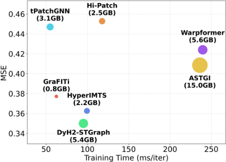
To evaluate the efficiency of DyH2-STGraph, we conduct a comparative analysis against the most competitive baselines on MIMIC-III dataset. From a data preprocessing perspective, these methods can be categorized as follows: (1) Canonical padding methods: Warpformer, (2) Patch-aligned padding method: tPatchGNN and Hi-Patch, (3) Non-padding methods: HyperIMTS, GraFITi, ASTGI and DyH2-STGraph. All models are evaluated based on their predictive accuracy (MSE), training time (ms/iter) and peak GPU memory usage. As illustrated in Figure 3, DyH2-STGraph achieves the state-of-the-art MSE, outperforming all baseline models while maintaining a highly competitive computational efficiency. Specifically, compared to heavy-duty architectures like ASTGI and Warpformer, DyH2-STGraph yields a significant reduction in training time from over 230 ms/iter to approximately 95 ms/iter, while requiring substantially less GPU memory (5.4 GB vs. 15.0 GB). Although lightweight models such as GraFITi and HyperIMTS exhibit lower memory footprints and training time, they suffer from higher prediction errors. Overall, DyH2-STGraph achieves a superior trade-off between predictive precision and computational efficiency. By avoiding the prohibitive costs of heavy-duty models and the fidelity loss of lightweight methods, it establishes a practical and robust paradigm for high-dimensional IMTS forecasting task.
5.6 Case Study
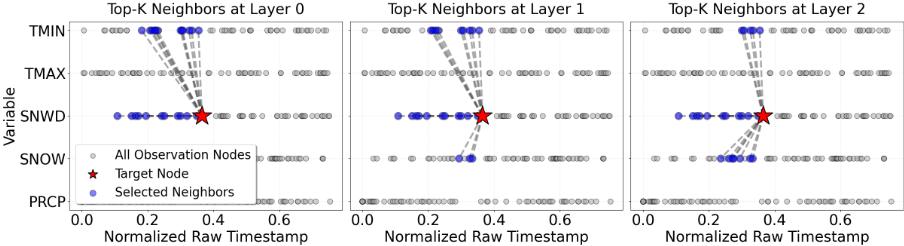
To qualitatively evaluate the dynamic neighbor selection in DyH2-STGraph, we conduct a case study on the USHCN dataset. We track the top-K neighbors of a target Snow Depth (SNWD) node (t ≈ 0.36) across successive layers, as illustrated in Figure 4. The visualization confirms that all selected neighbors strictly adhere to causal constraints. In Layer 0, the neighbors are primarily concentrated within the SNWD variable itself and a few Minimum Temperature (TMIN) nodes. As the network deepens, the target node broadens its receptive field to incorporate an increasing number of neighbors from the Snowfall (SNOW) variable, while the connections with TMIN relatively decreases. This evolution aligns with meteorological principles: snow depth is governed by both snowfall (SNOW) for accumulation and minimum temperature (TMIN) for melting effects, demonstrating the model's capacity to select relevant neighbors across variables. Meanwhile, the model's increasing focus on SNOW in deeper layers highlights its ability to prioritize the most direct physical drivers. In summary, the proposed neighbor selection mechanism allows the model to adaptively balance static spatiotemporal relations with dynamic feature similarity, enhancing its capacity to effectively capture crucial, fine-grained intervariable dependencies within the spatio-temporal graph.
6 Conclusion
This paper introduces DyH2-STGraph to address the fundamental challenges of IMTS forecasting. Representing variables as hypernodes and observations as spatio-temporal nodes allows the framework to preserve data fidelity, bypassing the distortions of traditional alignment-first strategies. By employing a three-fold decoupling strategy, the model captures intra-variable coarse-to-fine dependencies alongside multi-grained inter-variable correlations, overcoming the correlation loss prevalent in existing static models. Furthermore, the dynamic neighbor selection mechanism enables the model to adaptively capture evolving correlations as the network depth increases. Extensive experiments across four benchmark datasets demonstrate that DyH2-STGraph achieves state-of-the-art accuracy and stability, establishing a robust new paradigm for high-dimensional, asynchronous time series analysis.
Acknowledgments
This study is partially supported by National Natural Science Foundation of China (62276082), National Key R&D Program of China (2023YFC3502900), Shenzhen Science and Technology Research and Development Fund (KJZD20240903102802003), Shenzhen Science and Technology Research and Development Fund for Sustainable Development Project (GXWD20231128103819001, 20230706140548006) and Guangdong Provincial Key Laboratory Grant (2023B1212060076).
Contribution Statement
Xiaowei Yan and Zhuo Li contributed equally to this manuscript and are recognized as joint first authors.
@inproceedings{ijcai2026p573,
  title     = {Beyond Sequences: A Dynamic Hierarchical Heterogeneous Spatio-Temporal Graph for Irregular Multivariate Time Series Forecasting},
  author    = {Yan, Xiaowei and Li, Zhuo and Zhang, Junjie and Li, Bing and Yan, Jun and Tang, Buzhou},
  booktitle = {Proceedings of the Thirty-Fifth International Joint Conference on
               Artificial Intelligence, {IJCAI-26}},
  publisher = {International Joint Conferences on Artificial Intelligence Organization},
  editor    = {Diego Calvanese},
  pages     = {5146--5154},
  year      = {2026},
  month     = {8},
  note      = {Main Track},
  doi       = {10.24963/ijcai.2026/573},
  url       = {https://doi.org/10.24963/ijcai.2026/573},
}
TY - CPAPER TI - Beyond Sequences: A Dynamic Hierarchical Heterogeneous Spatio-Temporal Graph for Irregular Multivariate Time Series Forecasting AU - Yan, Xiaowei AU - Li, Zhuo AU - Zhang, Junjie AU - Li, Bing AU - Yan, Jun AU - Tang, Buzhou T2 - Proceedings of the Thirty-Fifth International Joint Conference on Artificial Intelligence, IJCAI-26 PB - International Joint Conferences on Artificial Intelligence Organization PY - 2026 SP - 5146 EP - 5154 DO - 10.24963/ijcai.2026/573 UR - https://doi.org/10.24963/ijcai.2026/573 ER -Copied
Machine-readable versions of this paper, for tools and AI agents:





