
Price of Fairness in Short-Term and Long-Term Algorithmic Selections
Proceedings of the Thirty-Fifth International Joint Conference on Artificial Intelligence. Main Track. Pages 635-643.
https://doi.org/10.24963/ijcai.2026/72
Keywords
- Planning and Scheduling: Theoretical foundations of planning
- AI Ethics, Trust, Fairnes: Societal impact of AI
- Constraint Satisfaction and Optimization: Constraint optimization problems
- AI Ethics, Trust, Fairnes: Fairness and diversity
Abstract
Algorithmic decision-making in high-stakes settings can have profound impacts on individuals and populations. While much prior work studies fairness in static settings, recent results show that enforcing static fairness constraints may exacerbate long-run disparities. Motivated by this tension, we study a stylized sequential selection problem in which a decision-maker repeatedly selects individuals, affecting both immediate utility and the population distribution over time. We introduce notions of group fairness for both the short and long term and theoretically analyze the trade-off between fairness and utility via the Price of Fairness (PoF). We characterize optimal and fair policies in the short term and show that the PoF can be large even when group distributions are nearly identical. In contrast, we show that long-term disparities can vanish under simple investment policies that achieve a low PoF. We also empirically validate these theoretical observations using both synthetic and real datasets.
- [Acharya et al., 2023] Krishna Acharya, Eshwar Ram Arunachaleswaran, Sampath Kannan, Aaron Roth, and Juba Ziani. Wealth dynamics over generations: Analysis and interventions. In SATML, pages 42-57, 2023.
- [Achiam et al., 2017] Joshua Achiam, David Held, Aviv Tamar, and Pieter Abbeel. Constrained policy optimization. In ICML, pages 22-31, 2017.
- [Altman, 1999] Eitan Altman. Constrained Markov Decision Processes. CRC Press, 1999.
- [Arunachaleswaran et al., 2021] Eshwar Arunachaleswaran, Sampath Kannan, Aaron Roth, and Juba Ziani. Pipeline interventions. In ITCS, pages 8:1-8:20, 2021.
- [Barocas et al., 2019] Solon Barocas, Moritz Hardt, and Arvind Narayanan. Fairness and Machine Learning: Limi- tations and Opportunities. fairmlbook.org, 2019.
- [Berk et al., 2021] Richard Berk, Hoda Heidari, Shahin Jab- bari, Michael Kearns, and Aaron Roth. Fairness in criminal justice risk assessments: The state of the art. Sociological Methods & Research, 50(1):3-44, 2021.
- [Bertsimas et al., 2011] Dimitris Bertsimas, Vivek Farias, and Nikolaos Trichakis. The price of fairness. Operations Research, 59(1):17-31, 2011.
- [Board of Governors of the Federal Reserve System, 2007] Board of Governors of the Federal Reserve System. Report to the congress on credit scoring and its effects on the availability and affordability of credit, 2007.
- [Calders and Verwer, 2010] Toon Calders and Sicco Verwer. Three naive bayes approaches for discrimination-free classification. Data Mining and Knowledge Discovery, 21(2):277-292, 2010.
- [Calvo-Fullana et al., 2024] Miguel Calvo-Fullana, Santiago Paternain, Luiz Chamon, and Alejandro Ribeiro. State aug- mented constrained reinforcement learning: Overcoming the limitations of learning with rewards. IEEE Transactions on Automatic Control, 69(7):4275-4290, 2024.
- [Celis et al., 2021] Elisa Celis, Anay Mehrotra, and Nisheeth Vishnoi. Fair classification with adversarial perturbations. In NeurIPS, pages 8158-8171, 2021.
- [Cheng et al., 2025] Zelei Cheng, Jiahao Yu, and Xinyu Xing. A survey on explainable deep reinforcement learning. CoRR, abs/2502.06869, 2025.
- [Chi et al., 2022] Jianfeng Chi, Jian Shen, Xinyi Dai, Weinan Zhang, Yuan Tian, and Han Zhao. Towards return parity in markov decision processes. In AISTATS, pages 1161-1178, 2022.
- [Corbett-Davies et al., 2017] Sam Corbett-Davies, Emma Pierson, Avi Feller, Sharad Goel, and Aziz Huq. Algo- rithmic decision making and the cost of fairness. In KDD, pages 797-806. ACM, 2017.
- [Corbett-Davies et al., 2023] Sam Corbett-Davies, Johann D. Gaebler, Hamed Nilforoshan, Ravi Shroff, and Sharad Goel. The measure and mismeasure of fairness. Journal of Ma- chine Learning Research, 24:312:1-312:117, 2023.
- [Cousins et al., 2024] Cyrus Cousins, Kavosh Asadi, Elita Lobo, and Michael Littman. On welfare-centric fair re- inforcement learning. Reinforcement Learning Journal, 3:1124-1137, 2024.
- [D'Amour et al., 2020] Alexander D'Amour, Hansa Srini- vasan, James Atwood, Pallavi Baljekar, D. Sculley, and Yoni Halpern. Fairness is not static: Deeper understand- ing of long term fairness via simulation studies. In FAccT, pages 525-534, 2020.
- [Davis et al., 2021] Jenny Davis, Apryl Williams, and Michael Yang. Algorithmic reparation. Big Data & Society, 8(2), 2021.
- [Deng et al., 2023] Zhun Deng, He Sun, Steven Wu, Linjun Zhang, and David Parkes. Reinforcement learning with stepwise fairness constraints. In AISTATS, volume 206, pages 10594-10618, 2023.
- [Ding et al., 2020] Dongsheng Ding, Kaiqing Zhang, Tamer Basar, and Mihailo Jovanovic. Natural policy gradient primal-dual method for constrained markov decision pro- cesses. In NeurIPS, 2020.
- [Ding et al., 2021] Dongsheng Ding, Xiaohan Wei, Zhuoran Yang, Zhaoran Wang, and Mihailo Jovanovic. Provably ef- ficient safe exploration via primal-dual policy optimization. In AISTATS, pages 3304-3312, 2021.
- [Donahue and Kleinberg, 2020] Kate Donahue and Jon Kleinberg. Fairness and utilization in allocating resources with uncertain demand. In FAccT, pages 658-668, 2020.
- [Dong et al., 2018] Jinshuo Dong, Aaron Roth, Zachary Schutzman, Bo Waggoner, and Zhiwei Steven Wu. Strate- gic classification from revealed preferences. In EC, pages 55-70, 2018.
- [Doroudi et al., 2017] Shayan Doroudi, Philip Thomas, and Emma Brunskill. Importance sampling for fair policy se- lection. In UAI, 2017. IJCAI
- [Eaton et al., 2025] Eric Eaton, Marcel Hussing, Michael Kearns, Aaron Roth, Sikata Bela Sengupta, and Jessica Sor- rell. Intersectional fairness in reinforcement learning with large state and constraint spaces. CoRR, abs/2502.11828, 2025.
- [Elzayn et al., 2019] Hadi Elzayn, Shahin Jabbari, Christo- pher Jung, Michael Kearns, Seth Neel, Aaron Roth, and Zachary Schutzman. Fair algorithms for learning in alloca- tion problems. In FAccT, pages 170-179, 2019.
- [Ghalme et al., 2022] Ganesh Ghalme, Vineet Nair, Vishakha Patil, and Yilun Zhou. Long-term resource allocation fair- ness in average markov decision process (AMDP) environ- ment. In AAMAS, pages 525-533, 2022.
- [Hardt et al., 2016a] Moritz Hardt, Nimrod Megiddo, Chris- tos Papadimitriou, and Mary Wootters. Strategic classi- fication. In Madhu Sudan, editor, ITCS, pages 111-122, 2016.
- [Hardt et al., 2016b] Moritz Hardt, Eric Price, and Nathan Srebro. Equality of opportunity in supervised learning. In NeurIPS, pages 3315-3323, 2016.
- [Hébert-Johnson et al., 2018] Úrsula Hébert-Johnson, Michael Kim, Omer Reingold, and Guy Rothblum. Multicalibration: Calibration for the (computationally- identifiable) masses. In ICML, pages 1944-1953, 2018.
- [Heidari and Kleinberg, 2021] Hoda Heidari and Jon Klein- berg. Allocating opportunities in a dynamic model of inter- generational mobility. In FAccT, pages 15-25, 2021.
- [Heidari et al., 2019a] Hoda Heidari, Michele Loi, Krishna Gummadi, and Andreas Krause. A moral framework for un- derstanding fair ML through economic models of equality of opportunity. In FAccT, pages 181-190, 2019.
- [Heidari et al., 2019b] Hoda Heidari, Vedant Nanda, and Kr- ishna Gummadi. On the long-term impact of algorithmic decision policies: Effort unfairness and feature segregation through social learning. In ICML, pages 2692-2701, 2019.
- [Hu and Zhang, 2022] Yaowei Hu and Lu Zhang. Achieving long-term fairness in sequential decision making. In AAAI, pages 9549-9557, 2022.
- [Jabbari et al., 2017] Shahin Jabbari, Matthew Joseph, Michael Kearns, Jamie Morgenstern, and Aaron Roth. Fairness in reinforcement learning. In ICML, pages 1617-1626, 2017.
- [Joseph et al., 2016] Matthew Joseph, Michael Kearns, Jamie Morgenstern, and Aaron Roth. Fairness in learning: Classic and contextual bandits. In NeurIPS, pages 325-333, 2016.
- [Kearns et al., 2018] Michael Kearns, Seth Neel, Aaron Roth, and Zhiwei Wu. Preventing fairness gerrymandering: Au- diting and learning for subgroup fairness. In ICML, pages 2569-2577, 2018.
- [Kleinberg and Raghavan, 2019] Jon Kleinberg and Manish Raghavan. How do classifiers induce agents to invest effort strategically? In EC, pages 825-844, 2019.
- [Liu and Hajiesmaili, 2025] Qingsong Liu and Mohammad Hajiesmaili. Online fair allocation of reusable resources. Proceedings of the ACM on Measurement and Analysis of Computing Systems, 9(2):1-46, 2025.
- [Liu et al., 2017] Yang Liu, Goran Radanovic, Christos Dim- itrakakis, Debmalya Mandal, and David C. Parkes. Cali- brated fairness in bandits. CoRR, abs/1707.01875, 2017.
- [Liu et al., 2018] Lydia Liu, Sarah Dean, Esther Rolf, Max Simchowitz, and Moritz Hardt. Delayed impact of fair machine learning. In ICML, pages 3156-3164, 2018. IJCAI
- [Liu et al., 2021] Tao Liu, Ruida Zhou, Dileep Kalathil, Pan- ganamala Kumar, and Chao Tian. Learning policies with zero or bounded constraint violation for constrained MDPs. In NeurIPS, pages 17183-17193, 2021.
- [Mansour et al., 2022] Yishay Mansour, Michal Moshkovitz, and Cynthia Rudin. There is no accuracy-interpretability tradeoff in reinforcement learning for mazes. CoRR, abs/2206.04266, 2022.
- [Menon and Williamson, 2018] Aditya Menon and Robert Williamson. The cost of fairness in binary classification. In FAccT, pages 107-118, 2018.
- [Mouzannar et al., 2019] Hussein Mouzannar, Mesrob Ohan- nessian, and Nathan Srebro. From fair decision making to social equality. In FAccT, pages 359-368, 2019.
- [Müller et al., 2024] Adrian Müller, Pragnya Alatur, Volkan Cevher, Giorgia Ramponi, and Niao He. Truly no-regret learning in constrained mdps. In ICML, 2024.
- [Rahmattalabi et al., 2021] Aida Rahmattalabi, Shahin Jab- bari, Himabindu Lakkaraju, Phebe Vayanos, Max Izenberg, Ryan Brown, Eric Rice, and Milind Tambe. Fair influence maximization: A welfare optimization approach. In AAAI, pages 11630-11638, 2021.
- [Rateike et al., 2024] Miriam Rateike, Isabel Valera, and Patrick Forré. Designing long-term group fair policies in dynamical systems. In FAccT, pages 20-50, 2024.
- [Reuel and Ma, 2024] Anka Reuel and Devin Ma. Fairness in reinforcement learning: A survey. In AIES, pages 1218- 1230. AAAI Press, 2024.
- [Salem et al., 2023] Tareq Si Salem, Georgios Iosifidis, and Giovanni Neglia. Enabling long-term fairness in dynamic resource allocation. In SIGMETRICS, pages 31-32, 2023.
- [Satija et al., 2023] Harsh Satija, Alessandro Lazaric, Matteo Pirotta, and Joelle Pineau. Group fairness in reinforcement learning. Transaction Machine Learning Research, 2023.
- [Silva et al., 2022] Andrew Silva, Rohit Chopra, and Matthew Gombolay. Cross-loss influence functions to ex- plain deep network representations. In AISTATS, volume 151, pages 1-17, 2022.
- [Sinha et al., 2023] Abhishek Sinha, Ativ Joshi, Rajarshi Bhattacharjee, Cameron Musco, and Mohammad Hajies- maili. No-regret algorithms for fair resource allocation. In NeurIPS, 2023.
- [Stoica et al., 2020] Ana-Andreea Stoica, Jessy Xinyi Han, and Augustin Chaintreau. Seeding network influence in biased networks and the benefits of diversity. In WWW, pages 2089-2098, 2020.
- [Tsang et al., 2019] Alan Tsang, Bryan Wilder, Eric Rice, Milind Tambe, and Yair Zick. Group-fairness in influence maximization. In IJCAI, pages 5997-6005, 2019. IJCAI
- [Wen and Topcu, 2018] Min Wen and Ufuk Topcu. Con- strained cross-entropy method for safe reinforcement learn- ing. In NeurIPS, pages 7461-7471, 2018.
- [Wen et al., 2021] Min Wen, Osbert Bastani, and Ufuk Topcu. Algorithms for fairness in sequential decision making. In AISTATS, pages 1144-1152, 2021.
- [Wu et al., 2025] Jiduan Wu, Rediet Abebe, Moritz Hardt, and Ana-Andreea Stoica. Policy design in long-run welfare dynamics. In ICLR, 2025.
- [Yin et al., 2023] Tongxin Yin, Reilly Raab, Mingyan Liu, and Yang Liu. Long-term fairness with unknown dynamics. CoRR, abs/2304.09362, 2023.
- [Zhang et al., 2020] Xueru Zhang, Ruibo Tu, Yang Liu, Mingyan Liu, Hedvig Kjellström, Kun Zhang, and Cheng Zhang. How do fair decisions fare in long-term qualifica- tion? In NeurIPS, 2020.
References were extracted automatically from the PDF and may contain errors.
Full text extracted automatically from the PDF; figures, tables and equations may differ. The PDF is the version of record.
1 Introduction
Motivated by the societal impact of algorithmic decisionmaking, prior work has documented discriminatory behaviors and proposed mitigatory and fairness-imposing algorithms across classification [Berk et al., 2021; Barocas et al., 2019], resource allocation [Elzayn et al., 2019; Donahue and Kleinberg, 2020; Tsang et al., 2019], and sequential decisionmaking [Reuel andMa, 2024]. However, this literature largely focuses on static or short-horizon settings, emphasizing immediate impacts while abstracting away long-term consequences.
In their seminal work, [Liu et al., 2018] showed that repeatedly enforcing static group-fairness notions from classification, such as demographic parity [Calders and Verwer, 2010] or equality of opportunity [Hardt et al., 2016b], can lead to stagnation and exacerbate group disparities when decisions influence the environment, sometimes even performing worse than simple utility maximization. Since then, various long-term fairness notions and algorithms-including those based on reinforcement learning-have been proposed to mitigate these effects [Wen et al., 2021; Chi et al., 2022]. However, existing results either establish strong impossibility or incompatibility results for jointly achieving fairness and high utility [Jabbari et al., 2017; Doroudi et al., 2017], or lack theoretical guarantees for optimal fair policies and thus offer no formal characterization of the fairness-utility tradeoff [Wen et al., 2021; Hu and Zhang, 2022].
→The full version of this paper with the appendix is available here: https://arxiv.org/abs/2605.06227.
Our Results and Contributions. Motivated by this gap, we study a stylized selection problem in which a decision-maker (e.g., a financial institution) sequentially selects a set of individuals (e.g., to lend money) in each round. In our model, individuals belong to different groups and are represented by single-dimensional features (e.g., credit score). These decisions and their consequences (e.g., default or full payback) affect the decision-maker's utility and the distribution of individuals for future rounds. Given the potential disparity in the distributions, the decision-maker's selection policy can favor specific groups or individuals, raising concerns about unfairness and disparate treatment or impact. Furthermore, these disparities can worsen over time as population distribution evolves. We propose a new notion of group fairness, both for the short and the long terms, requiring the group difference between the means of score distributions to be bounded.
Our goal is to understand the theoretical foundation of the trade-off between fairness violations and utility maximization in both the short and long terms. To this end, we define the notion of Price of Fairness (PoF) for this domain, capturing the cost of utility due to fairness constraints. We characterize optimal and fair short-term selection policies and show that threshold-based policies can achieve optimal utility. We then show that in the short term, the PoF can be arbitrarily high even when the groups have very similar initial distributions.
The characterization of optimal and fair policies becomes significantly more complex in the long term, where current decisions interfere with future states of the population. In the single-step setting, fairness constraints often force a strict trade-off between utility and equity. However, we show that in the multi-step setting, this trade-off is largely an artifact of the short horizon. We analyze a class of long-term investment policies, i.e., simple investment strategies that prioritize score improvement and prove that they guarantee a low PoF. We also empirically validate these theoretical observations using both synthetic data and real-world FICO credit score datasets.
2 RelatedWork
We focus on the closest related work. See Appendix A.
Fairness in Sequential Decision-Making. Fairness in dynamic and repeated decision-making has been widely studied; see [Reuel and Ma, 2024]. Early work considers stationary bandit settings [Liu et al., 2017; Joseph et al., 2016]. In general MDPs, [Jabbari et al., 2017] formalize meritocratic fairness and show its incompatibility with utility maximization, a phenomenon also noted in [Doroudi et al., 2017]. Subsequent work on fair reinforcement learning imposes population-level constraints on average reward or return [Wen et al., 2021; Chi et al., 2022; Hu and Zhang, 2022], emphasizing allocative equality. Instead, we focus on restorative justice and substantive equality (see Remarks 1-2). Other related approaches include state-visit constraints [Ghalme et al., 2022], minimax fairness [Eaton et al., 2025], and welfare-based objectives [Cousins et al., 2024]; see also [Satija et al., 2023; Deng et al., 2023; Zhang et al., 2020; Yin et al., 2023]. Our notion of fairness is inspired by state-based constraints [Ghalme et al., 2022], but we focus on characterizing optimal fair policies and analyzing the fairness-utility tradeoff. Unlike intervention-based approaches in dynamical systems [Rateike et al., 2024], we quantify the Price of Fairness in a fixed environment and show it vanishes under a class of investment policies. Our work is distinct from fair division [Salem et al., 2023; Liu and Hajiesmaili, 2025; Sinha et al., 2023].
Fairness in Stylized Dynamic Settings. Fairness has also been studied in stylized dynamic models. [Arunachaleswaran et al., 2021] analyzes a multi-layer life-stage model with costly interventions in transition dynamics (see also [Acharya et al., 2023]). Intergenerational dynamics driven by wealth and talent are studied in [Heidari and Kleinberg, 2021]. In a continuous-time model, [Mouzannar et al., 2019] characterizes when affirmative action constraints improve long-run outcomes despite short-term costs. Simulation-based studies appear in [D'Amour et al., 2020], while causal distribution shifts are modeled in [Hu and Zhang, 2022]. Finally, [Wu et al., 2025] identifies conditions under which Rawlsian policies outperform utilitarian policies in the long run.
3 Single-step Setting
3.1 Model and Notation
We start by presenting our stylized model of sequential decision-making, which mainly follows the model proposed in the seminal work of [Liu et al., 2018]. We assume the information about each individual is aggregated using a onedimensional score x in a bounded range X (e.g., X can be the credit scores in lending). The score can be interpreted as an indication of an individual's perceived ability, with higher scores being more desirable. We assume individuals belong to two groups: g ↑ ¶A,B♦. We use DA and DB to denote the distributions over scores for each group, capturing the variation in scores within each group. We use θA and θB to denote the mean score for each group. Without loss of generality, we assume θA ↓ θB and, hence, group A to have an advantage over group B. We use wg to denote the fraction of the population that belongs to group g, so wA + wB = 1.
We assume the decision-maker deploys a group-dependent policy ω : X ↔ g ↗ [0, 1] to select individuals with a given score from each group, interpreted as the selection probability of an individual with a score x within each group. We use ωA and ωB to denote the policies corresponding to each group, hence, ω = ¶ωA, ωB♦. When selected, each individual with a score x has a group-agnostic probability of success denoted by p : X ↗ [0, 1]. Similar to [Liu et al., 2018], we make the following assumption on p, demonstrating that success probabilities are positively correlated with the scores.
Assumption 1 ([Liu et al., 2018]). p : X ↗ [0, 1] is a monotonically increasing function of the score x.
When an individual with score x is selected, the decisionmaker receives a fixed profit of U + ↓ 0 if the individual succeeds (which happens with probability p(x)). Otherwise, the decision-maker incurs a cost of U → < 0 (which happens with probability 1 ↘ p(x)). Thus, for a selected individual with score x, the expected utility u : X ↗ R of the decisionmaker can be written as E [u(x)] = p(x)U + +(1 ↘ p(x)) U →. The success of the individual can also impact their score. In particular, we assume, upon success, the score increases by C + ↓ 0 (which happens with probability p(x)). Otherwise, the score decreases by C → < 0 (which happens with probability 1 ↘ p(x)). 1 Thus, the expected change ! : X ↗ R in score for an individual with score x can be written as E[!(x)] = p(x)C + + (1 ↘ p(x))C →. For individuals who are not selected, we assume the score to remain the same and the decision-maker to receive 0 utility.
By Assumption 1, both the expected utility and the expected score change are monotone functions of the score. Similar to [Liu et al., 2018], we assume the utility function for individuals is stricter than the score change function.
Assumption 2 implies that if E[u(x)] ↓ 0 then E[!(x)] ↓ 0, which is an important property for the non-existence of extractive (exploitative) outcomes, where the decision-maker can profit from the long-term decrement of the individual scores. We study the relaxation of this assumption in Section 5. See Definition 2 and Observation 1 for more details.
An instance I of the selection problem is determined by the description of X, DA, DB, wA, wB, p, U +, U →, C +, and C →. The expected utility for any selection policy ω is defined as
The decision-maker's goal in the single-step setting is to compute an optimal policy ω maximizing the total expected utility:
where OPT(I) denotes the utility of the optimal policy.
3.2 Fairness Definition
The groups start with different distributions of scores, and the decision-maker's policy can further exacerbate this difference, raising concerns about disparate impact and unfairness of the selection policy. It is well known that static intervention policies such as equal selection rates (statistical parity) or equal selection rates conditioned on qualification status (equality of opportunity) can further worsen the discrepancies between the groups [Liu et al., 2018; Zhang et al., 2020]. To alleviate this, inspired by [Liu et al., 2018], we define a fairness constraint on the decisionmaker's policy requiring the difference between the means of the distributions for different groups after deploying the policy to be bounded by a parameter ε ↓ 0. Formally, let ϑ = θA ↘ θB ↓ 0 denote the mean score difference between the two groups, capturing the initial disparity. Also let
1 Since the scores are bounded, the updated scores should be projected/clipped to guarantee that they fall inside of X.
| Assumption | Justification |
|---|---|
| Assumption 1 | Same as [Liu et al., 2018], higher score individuals have higher chances to succeed. |
| Assumption 2 | Same as [Liu et al., 2018], the utility function for individuals is stricter than the score change function. |
for g ↑ ¶A,B♦ to denote the mean after deploying ω. Therefore, ϑ↔ (ω) = ♣θ↔A(ωA) ↘ θ↔B (ωB)♣ represents the postdeployment difference in the means. We next propose our fairness definition in the single-step setting.
Definition 1. A policy ω = ¶ωA, ωB♦ satisfies ε-fairness for some ε ↓ 0 if ϑ↔ (ω) ≃ ε.
The parameter ε controls the degree of mean disparity after policy deployment, and smaller ε values correspond to more restrictive policies. When it is clear from the context, we drop the dependency of θ↔g (ωg) on ωg and simply write θ↔g .
Remark 1. Our notion of fairness focuses on the states (scores) as opposed to outcomes (utilities) [Chi et al., 2022], preventing negative feedback loops that [Liu et al., 2018] have warned about. It also enforces restorative justice [Davis et al., 2021] and substantive equality of opportunity [Heidari et al., 2019a], requiring the decision-maker to invest in the group with a lower average score. See Section 4.
Remark 2. Given Assumption 1 on the direct correlation of scores and qualification status, the closeness of average scores, indirectly, enforces the closeness of average qualification status between the groups. Similar to [Liu et al., 2018], we define fairness using the scores, i.e., the scores are changing, and the score-dependent qualification scores remain fixed. See [Zhang et al., 2020] that takes the alternative approach, where scores are fixed, and the qualification statuses are changing.
An optimal fair policy, for instance I in the single-step setting, is a policy ω that maximizes the decision-maker's expected utility subject to satisfying the fairness constraint in Definition 1. Formally, this can be written as follows:
We use Fair-OPT(I) to denote the utility of the optimal fair policy. In the multi-step setting, the decision-maker selects individuals repeatedly over rounds, causing the scores to change in each step. We discuss that setting in Section 4.
3.3 Characterization of the Optimal Policies
To study the short-term effects of selection policy, in this section, we start by characterizing the optimal policy (Proposition 1) and optimal fair policies (Theorem 1) in the single-step setting. We first define the categories of the individual scores based on the expected utility and score change.
Definition 2. For any score x ↑ X, we say x is in one of the following categories:
- Profitable and Improving: We say x is in category 1, denoted as x ↑ C1, if E [!(x)] ↓ 0 and E [u(x)] ↓ 0.
- Extractive Candidates: We say x is in category 2, denoted as x ↑ C2, if E [!(x)] < 0 and E [u(x)] ↓ 0.
- Investment Candidates: We say x is in category 3, denoted as x ↑ C3, if E [!(x)] ↓ 0 and E [u(x)] < 0.
- Unprofitable and Degrading: We say x is in category 4, denoted as x ↑ C4, if E [!(x)] < 0 and E [u(x)] < 0.
We want to argue that the optimal (utility-maximizing) policy has to be a threshold policy. To this end, we start by formally defining threshold policies.
Our first crucial observation is that under Assumption 2, the exploitative outcomes do not exist, i.e., we do not have category 2 with E [!(x)] < 0 and E [u(x)] ↓ 0. See Appendix B. Observation 1. Under Assumption 2, the set of Extractive Candidates (C2) is empty, i.e., C2 = ⇐.
Definition 3 (Threshold policy). A policy ω is a threshold policy if there exists x↗ ↑ X and ϖ ↑ [0, 1] such that
In Definition 3, x↗ represents the threshold score, and ϖ is the fraction of selected individuals at the threshold score. Threshold policies are desirable since they offer simplicity and interpretability [Corbett-Davies et al., 2023]. Proposition 1 states that the optimal policy selects only individuals with positive expected utility, exactly characterized by category 1.
Proposition 1 ([Liu et al., 2018]). Under Assumption 1, the optimal policy in the single step is a group-agnostic threshold policy that selects all the individuals in category 1, i.e., individuals with score x such that p(x) ↓ ↘U →◁(U + ↘ U →).
We next show that optimal fair policies, when they exist, are also thresholding policies. However, unlike optimal policies, the threshold can be different for each group.
Theorem 1. Suppose the optimization problem in Equation 4 has a feasible solution. Under Assumptions 1 and 2, in the single-step setting, there exists an optimal fair policy that is a threshold policy for each group.
This observation is also consistent with prior work [CorbettDavies et al., 2023]. See Appendix B for proof.
3.4 Price of Fairness
We next study the relationship between the expected utility of optimal and optimal fair policies in the single-step setting. We measure the cost of enforcing the fairness constraint as the fraction of expected utility retained by the optimal fair policy compared to the optimal policy in the worst case over all instances. In line with prior work studying fairness in different decision-making settings [Bertsimas et al., 2011; Menon and Williamson, 2018; Elzayn et al., 2019; Donahue and Kleinberg, 2020], we call this notion price of fairness.
Definition 4. The Price of Fairness (PoF) is defined as:
The PoF is in [0, 1], and higher PoF values mean that enforcing fairness requires a higher degree of utility degradation. Hence, lower values of the price of fairness are more desirable. In Theorem 2, an ε-dependent lower bound on PoF indicates that in the worst-case, the PoF can get arbitrarily close to 1 in the single-step setting when ε goes to 0.
Theorem 2. Suppose X = [0, 1]. Then, in the single-step setting, PoF ↓ 1 ↘ O(ε).
The proof relies on creating a family of instances I and a characterization of the optimal and optimal fair policies for this family. We defer the proof to Appendix B. To show a large PoF, the proof relies on constructing an instance in which the population distributions are very different (i.e., the total variation distance of the two distributions is 1). This raises a natural question: can high PoF be avoided if the distributions are more similar (e.g., have a smaller total variation distance)? Before answering this question, we require the following definition.
Definition 5. A policy ω is non-degrading if ω(x) = 0, ⇒x ↑ C4, i.e., no allocation to individuals in C4 category.
Recall that an individual x belongs to category 4 if E[u(x)] < 0, E[!(x)] < 0. A population-degrading policy selects individuals that not only impose negative expected utility but also degrade population scores. It is known that equality-enforcing fairness notions (such as our notion) can lead to population degradation [Rahmattalabi et al., 2021; Stoica et al., 2020]. Our next result shows that it is not possible to avoid high PoFs for all non-degrading policies.
Theorem 3. For any ϱ > 0, in the single-step setting, there exists an instance such that the total variation distance between DA and DB is at most ϱ, but the PoF is 1 ↘O(ε).
See Appendix B for proof. Finally, in Proposition 3 (Appendix B), we provide sufficient conditions where more favorable PoFs are achievable. These results indicate that for the single-step setting, in general, the PoF can be quite large.
4 Multi-step Setting
We now focus on the long-term effects of the selection policy by studying the multi-step setting. In this setting, the decision-maker makes selections sequentially for T rounds. The decisions in the previous steps 1, ▷ ▷ ▷ , t ↘ 1 will affect the distribution at time step t. The decision-maker likes to maximize the total utility over all time steps. We show that, unlike in the single-step setting, where the PoF could be high, we can obtain a low PoF using simple investment policies.
4.1 Model and Notation
For simplicity, we assume the scores are integers from 0 to xmax. We work extensively with the categories of the scores as defined in Definition 2. For convenience, we use g ↑ ¶A, B♦ and c ↑ ¶1, 3, 4♦ to refer to individuals in each group and category, respectively. For example, we use A⇑C1 to denote individuals from group A that belong to category C1. For each category c and group g, we define "cg and θcg as the total and average scores of the specific category c and group g, i.e.,
Let T be the total number of time steps. We use D(t) g to denote the distribution of the scores for group g ↑ ¶A,B♦ at step t. The multi-step allocation model is a stochastic process, where the decision maker selects a sequence of policies #T = ¶ω(t) ♦Tt=1 . We also track the change of scores during the stochastic process: let x be any score at time step 1, the notation G(x)t is defined as the set of scores after evolving for t steps 2 . The multi-step utility can be written as follows.
where the equality holds due to the linearity of expectation. However, note that the random variables in different steps are not independent since the past realization will affect ωt and Dt (see Appendix C.1 for more insight about the dependency).
To define a multi-step analog of Definition 1 for fairness, we could similarly define θ↔g (#t) as the expected average score for group g ↑ ¶A,B♦ for the t-th time step, and ϑ↔ (#t, t) = ♣θ↔A(#t) ↘ θ↔B (#t)♣.
We restrict our attention to rational (non-degrading) policies and introduce the multi-step version of the non-degrading policy, which generalizes Definition 5.
Assumption 3. A policy ω is rational (non-degrading) in the multi-step setting, if for all t ↑ [T ], g ↑ ¶A, B♦ and x ↑ C4, ω(t) g (x) = 0.
Assumption 3 says that no policy will allocate resources to an individual expected to be unprofitable in both the short and long terms, implying that the decision-maker is rational. Our next assumption characterizes the advantage group A over B.
Assumption 4. We assume that the scores for group A in categories C1 and C3 are greater than the scores from the same categories for group B by a positive value ς > 0, i.e., "C1 A +"C3 A B +"C3 B
Assumption 4 states that the advantage of group A is not due to a strange scenario where the group has no "real advantage"
2 More formally, G(x)t is a realization of the random variable denoting the set of score. See Appendix C.1 for a rigorous definition.
| Assumption | Setting | Justification |
|---|---|---|
| Assumption 3 | Single & Multi- opportunity | The decision-maker is rational and avoids individuals expected to yield net utility losses in both the short and long term. |
| Assumption 4 | Single & Multi- opportunity | Ensures Group A's advantage stems from potentially profitable candidates rather than simply having fewer unprofitable ones. |
| Assumption 5 | Single- opportunity | Models "stability" where profitable candidates are trustworthy, effectively controlling the variance of the score trajectory. |
| Assumption 6 | Single- opportunity | Aligns with natural distributions (e.g., logistic) where success probability improves rapidly in low-to-mid score ranges. |
| Assumption 7 | Multi- opportunity | Reflects real-world scoring systems (e.g., FICO) where scores are treated as discrete integers and updates occur in integer increments. |
among the individuals who could get allocations, and it simply has a smaller number of individuals with very bad scores.
We consider two settings for multi-step allocation: the single-opportunity setting, where the decision-maker adjusts scores based on a single outcome, and the multi-opportunity setting, where the decision-maker modifies scores only after the outcomes of multiple independent decisions. Table 2 provides a summary of the assumptions used in this section.
Technical Overview. At a high level, the reason we can obtain low PoF is due to the positive drift for individuals in categories C1 and C3 and the existence of the xmax score. If we only look at the expectation, the intuition for low PoF is straightforward and clean: for any score x ↑ C1 ⇓ C3, we have E [!(x)] > 0 then, when T ↗ ⇔, the scores for both advantaged and disadvantaged groups are expected to hit xmax. Therefore, unless the gap between the groups is induced by C4 (which is a very strange situation since the advantaged group has no "real advantage"), the gap between the mean scores should decrease. Furthermore, for the utility, the decisionmaker only pays the "burn-in" part for individuals in C1 ⇓ C3 to reach xmax; and afterwards, the decision-maker is expected to get the maximum possible utility. This summarizes the intuitive reason for the PoF to be low.
The actual analysis, however, is much more challenging and complicated. The challenge lies in the expectation vs. realization. Since multi-step allocation is a stochastic process, the realization of the randomness in the previous steps interferes with the current and future steps. An adversarial case can be as follows: in one step, many scores in C3 drop to C4, and the high expected score and utility can never materialize.
We overcome the challenge in two ways: i) for the singleopportunity setting, we introduce additional realistic assumptions to bound the variance of the scores; and ii) in the multiopportunity setting, we directly leverage the multiple trials to introduce concentration. The analysis in the single-opportunity setting is perhaps more intellectually stimulating. Here, we only assume the failure probability for individuals in C1 ⇓ C3 is bounded, and the success probability increases fast in the low-to-mid score ranges-both are considered common in practice. We explicitly track the change of scores by bounding the probability of "failure to increase", and we prove that the set of scores that cannot increase forms a geometrically decreasing series with high probability. Hence, we can "peel off" this small fraction of "bad scores", and use the scores that kept increasing to argue both improved fairness and low PoFs.
4.2 Price of Fairness
Single-opportunity Setting. In the single-opportunity setting, the decision-maker adjusts scores every time after an individual succeeds or fails. In this setting, with specific but natural assumptions, we can achieve fairness with low PoF as T increases. We first introduce the following assumptions used exclusively for the single-opportunity setting.
Assumption 5. For any x ↑ C1 ⇓ C3, we assume the probability of failure is at most ε N·xmax for sufficiently large constant N, i.e., 1 ↘ p(x) ≃ ε N·xmax . Here, ς is the parameter in Assumption 4, and xmax is the maximum score.
Furthermore, in the single-opportunity setting, we control the variance of the realization of the score by adding another assumption on the failure probability.
Assumption 6. We assume for any score x ↑ X , 1 ↘ p(x + C +) ≃ 13 · (1↘p(x)). Furthermore, we assume the individuals with the maximum score always succeed, i.e., p(xmax) = 1.
In practice, Assumption 6 holds when the probability of success increases drastically during the low-to-mid score ranges. One natural family of distributions in this regime is logistic distributions, and we provide a justification in Appendix C.2. We show a structural lemma that, if we keep selecting individuals in C1 ⇓ C3, we will have a good probability to receive a "cascading" effect for a majority of such individuals. This is stated in Lemma 2 (proof in Appendix C). Recall that G(x)t is the set of scores starting from x and evolving till t-th step.
Lemma 2. Suppose for any x ↑ C1⇓C3, the success probability p(x) satisfies p(x) ↓ 1 ↘ pfail. Then, under Assumption 6, with probability at least 99◁100, for all but at most O(pfail) fraction of scores in G(x)(t) , we have
∣∣¶x ↑ G(x)t ♣ x = xmax♦∣∣ ↓ (1 ↘O(pfail)) · ∣∣G(x)t ∣∣ . We now introduce the main results for the multi-step singleopportunity setting. We argue that, unlike the single-step setting, for the multi-step setting, if the number of steps is sufficiently large, we could use the following simple long-term investment policy to simultaneously satisfy fairness and obtain low PoF. This is stated in Theorem 4 (proof in Appendix C).
A simple long-term investment policy.
- Select individuals in both A and B groups who have always succeeded in the previous round (with Assumption 3, this is a subset of individuals in C1 and C3).
Theorem 4. Assume Assumptions 3, 4, 5, and 6 hold. Then, with probability at least 99◁100, for sufficiently large T, the long-term investment policy guarantees ϑ↔ (T ) < ♣θA ↘θB♣ ↘ ς◁2, where ♣θA ↘θB♣ is the initial gap of the mean scores of the groups, and ς is the parameter in Assumptions 4 and 5.
Furthermore, we have that limT≃⇐ PoF = O(pfail) as long
The conditions in Theorem 4 implies that the statement holds for ε ↓ max¶θC4 A , θC4 B ♦ + ς as well, although the statement is much weaker.
Multi-opportunity Setting. We further investigate a different setting, where the decision-maker will keep selecting for multiple times before committing to a decision that would be used for the rest of the time steps. We will show that in this setting, the PoF goes to 0 with high probability with assumptions much weaker than Assumptions 5 and 6. First, we formally define the multi-opportunity setting in the multi-step setting.
Definition 6. Let x(t) be any score at time step t. In the multistep setting with number of opportunities m, the decisionmaker selects an individual m times, and makes selection decisions after observing all outcomes of the m selections.
Let gsuccess be the fraction of the times the individual succeeds.
Note that the expected score change remains the same:
We also introduce a much milder assumption about the expectation of the change of score.
Assumption 7. For any score x ↑ X, the expectation of the change of scores, i.e., E [!(x)], is a positive integer.
In the multi-opportunity setting, we could simply select all individuals in C1 and C3 to get a low PoF.
An even simpler long-term investment policy.
- Select individuals from categories C1 and C3 in both groups A and B.
We formally show the guarantees for the "even simpler investment policy" as follows. Note that the quantifiers here are different from those of Theorem 4: we first fix the time horizon T before giving the parameters for the multi-opportunity setting. We defer the proof to Appendix C.
Theorem 5. Assume Assumptions 3, 4, and 7 hold. For any sufficiently large T and ϑ > 0, suppose we have m ↓ 5(C + ↘C →) · logT in the multi-opportunity setting. Then, with probability at least 99◁100, the even simpler long-term investment policy guarantees ϑ↔ (T ) < ϑ and PoF = 0 as long as ε ↓ max¶θC4 A , θC4 B ♦.
5 Experiments
Dataset and Implementation Details. We experimented on two datasets. One is a synthetic dataset with scores drawn from two Gaussian distributions with different means but the same variance, post-processed to integers in 0 to 100. The other is a real-world dataset of FICO credit scores [Board of Governors of the Federal Reserve System, 2007], also used in [Hardt et al., 2016b; Liu et al., 2018]. We selected individuals labeled as White or Black to form groups A and B. We used different parameter choices to define instances, and these choices are described in each experiment. In all experiments, the p(x) increases linearly in the range of scores from 0 to 1. To solve for the optimal fair policy in the single-step, we used an LP solver since the optimization in Equation 4 is linear in ω. Motivated by Proposition 1, we also implemented an algorithm that searches over all possible thresholds for each group. See Appendix D. Our code is available here.
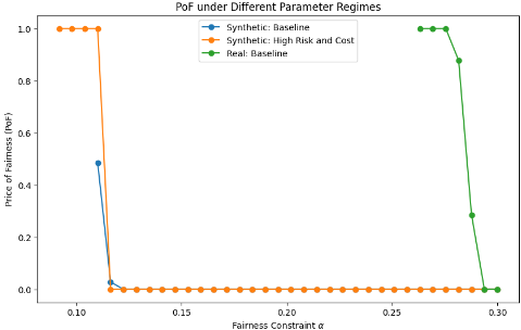
Single-step Results. As our first experiment, we study the PoF on our two datasets. For each dataset, we use a baseline set of parameters to generate an instance. For the synthetic experiments, we also generate an instance with high cost and risk, which, compared to the baseline, has a higher U → and C → but the same U + and C +. All instances satisfy Assumption 2. See Appendix D for more details. Figure 1 plots the PoF for each choice as a function of ε times the range of the score. So ε = 0 corresponds to enforcing exact mean-equality and ε = 1 corresponds to no constraints on the means. If for any given ε, no fair policy is found, there are no corresponding points on the curves. We observe that a lower ε is required for synthetic data compared to real data to achieve 0 PoF. In Appendix D.2, we show that the simple thresholding algorithm is also effective when Assumption 2 is violated. Multi-step Results. We investigate the long-term dynamics of fairness and utility in a sequential selection process, modeled as a feedback loop where algorithmic decisions influence future population states. For this experiment, we sample a population of N = 1, 000, 000 agents drawn from the baseline synthetic distribution and analyze how the scores evolve over a horizon of T = 100 steps under different policies. At each time step, a policy selects a subset of agents, who then succeed or fail. We evaluate four distinct policies: a myopic policy maximizing immediate utility, our investment policy maximizing expected score growth, a threshold policy constrained by a relaxed fairness gap (ε = 0.01), and a zero-gap LP policy enforcing strict equality of expected future means via linear programming. The myopic and investment policies prioritize aggregate utility and capability growth, respectively, without explicit distributional constraints. In contrast, the threshold policy introduces a soft constraint, optimizing utility while bounding the expected inter-group mean score difference. The zero-gap LP approach represents a hard constraint, solving for selection probabilities ωg(x) that strictly force the expected fairness gap to zero at each step. These policies allow for an analysis of the trade-offs between maximizing total utility and achieving fairness in the multi-step setting.
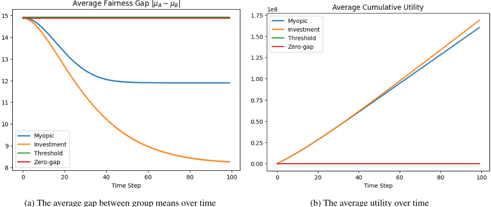
Results are summarized in Figure 2: left and right panels track the difference between the mean of the groups and total utility obtained by each of the policies, averaged over 5 runs. We observe that our proposed investment policy is not only effective in reducing unfairness but also achieves higher utility compared to all the baselines. The experiments also show that our theory is fairly robust, as the p(x) distribution does not satisfy Assumption 6, yet the empirical PoF is still small.
6 Discussion and FutureWork
A central contribution of our framework is reframing the price of fairness (PoF) from a static penalty to a dynamic investment. Whereas prior work (e.g., [Bertsimas et al., 2011]) views PoF as an inherent utility loss, our multi-step analysis shows that this loss is largely transient, i.e., a down payment that rehabilitates the score distribution of the disadvantaged group. Our theorems formalize the resulting patience premium, indicating that the apparent conflict between fairness and utility is partly driven by short horizons: under long-term greedy policies, fairness constraints eventually align with profit maximization, provided the allocator can absorb the initial loss. Our fairness notion minimizes gaps between group means. While analytically convenient, such mean-based metrics capture only average outcomes and do not ensure individual-level fairness, nor do they preclude fairness gerrymandering.
There are several directions to extend our work. First, individuals are often represented by high-dimensional features with unobservable attributes, and deployable policies may be significantly more complex. Moreover, feature changes may arise not only from practice but also from improvement [Kleinberg and Raghavan, 2019; Heidari et al., 2019b] or manipulation and gaming [Hardt et al., 2016a; Dong et al., 2018]. Second, stronger notions of fairness could require closeness of entire distributions (e.g., via total variation or earth mover's distance) or enforce fairness at every time step rather than only at the end [Jabbari et al., 2017]. Third, we assume the decision-maker can use sensitive attributes, although optimal fair threshold policies may be group-specific when feature distributions differ [Corbett-Davies et al., 2017]. In practice, sensitive attributes may be unavailable or prohibited [Celis et al., 2021], and populations often consist of multiple, intersecting protected groups [Kearns et al., 2018; H´ebert-Johnson et al., 2018]. Finally, many applications face resource constraints (e.g., college admissions) not captured by our model. We leave these questions for future work.
Acknowledgments
We thank Alvand Vahediahmar for discussions during the early stages of this work. The authors used Gemini Pro as an aid in writing code, which was reviewed and edited by the authors.
@inproceedings{ijcai2026p72,
  title     = {Price of Fairness in Short-Term and Long-Term Algorithmic Selections},
  author    = {Jabbari, Shahin and Wang, Chen},
  booktitle = {Proceedings of the Thirty-Fifth International Joint Conference on
               Artificial Intelligence, {IJCAI-26}},
  publisher = {International Joint Conferences on Artificial Intelligence Organization},
  editor    = {Diego Calvanese},
  pages     = {635--643},
  year      = {2026},
  month     = {8},
  note      = {Main Track},
  doi       = {10.24963/ijcai.2026/72},
  url       = {https://doi.org/10.24963/ijcai.2026/72},
}
TY - CPAPER TI - Price of Fairness in Short-Term and Long-Term Algorithmic Selections AU - Jabbari, Shahin AU - Wang, Chen T2 - Proceedings of the Thirty-Fifth International Joint Conference on Artificial Intelligence, IJCAI-26 PB - International Joint Conferences on Artificial Intelligence Organization PY - 2026 SP - 635 EP - 643 DO - 10.24963/ijcai.2026/72 UR - https://doi.org/10.24963/ijcai.2026/72 ER -Copied
Machine-readable versions of this paper, for tools and AI agents:





