
HieraMix: A Hierarchical MLP-Mixer for Large-Scale Traffic Forecasting
Proceedings of the Thirty-Fifth International Joint Conference on Artificial Intelligence. AI4Tech: AI Enabling Technologies. Pages 6555-6563.
https://doi.org/10.24963/ijcai.2026/729
Keywords
- Domain-specific AI4Tech: AI4Transport
Abstract
Traffic forecasting task is significant to modern urban management. Recently, there is growing attention on large-scale forecasting, as it better reflects the complexity of real-world traffic networks. However, existing models often exhibit quadratic computational complexity, making them impractical for large-scale real-world scenarios. In this paper, we propose a novel framework, Spatio-Temporal Hierarchical Mixer (HieraMix), which leverages an all-MLP architecture for efficient and effective large-scale traffic forecasting. HieraMix employs a hierarchical spatiotemporal mixing block to extract multi-resolution features through bottom-up aggregation and top-down propagation. Furthermore, an adaptive region mixer generates transformation matrices based on regional semantics, enabling our model to dynamically capture evolving spatiotemporal patterns for different regions. Extensive experiments conducted on four large-scale real-world datasets demonstrate that the proposed method not only achieves state-of-the-art performance but also exhibits competitive computational efficiency.
- [Bai et al., 2020] Lei Bai, Lina Yao, Can Li, Xianzhi Wang, and Can Wang. Adaptive graph convolutional recurrent network for traffic forecasting. Advances in neural infor- mation processing systems, 33:17804-17815, 2020.
- [Chen et al., 2023] Si-An Chen, Chun-Liang Li, Nate Yo- der, Sercan Ö. Arik, and Tomas Pfister. Tsmixer: An all-mlp architecture for time series forecasting. CoRR, abs/2303.06053, 2023.
- [Dauphin et al., 2017] Yann N. Dauphin, Angela Fan, Michael Auli, and David Grangier. Language modeling with gated convolutional networks. In ICML, volume 70 of Proceedings of Machine Learning Research, pages 933- 941. PMLR, 2017.
- [Deng et al., 2025] Zerong Deng, Liangzhe Han, Tongyu Zhu, Ziqi Miao, Yi Xu, and Leilei Sun. Urban in-context learning: A new paradigm for urban indicator prediction. In Proceedings of the 34th ACM International Conference on Information and Knowledge Management, pages 553- 563, 2025.
- [Duan et al., 2024] Wenying Duan, Tianxiang Fang, Hong Rao, and Xiaoxi He. Pre-training identification of graph winning tickets in adaptive spatial-temporal graph neural networks. In Proceedings of the 30th ACM SIGKDD Con- ference on Knowledge Discovery and Data Mining, pages 701-712, 2024.
- [Fang et al., 2021] Zheng Fang, Qingqing Long, Guojie Song, and Kunqing Xie. Spatial-temporal graph ODE net- works for traffic flow forecasting. In KDD, pages 364-373. ACM, 2021.
- [Fang et al., 2024] Yuchen Fang, Yuxuan Liang, Bo Hui, Zezhi Shao, Liwei Deng, Xu Liu, Xinke Jiang, and Kai Zheng. Efficient large-scale traffic forecasting with trans- formers: A spatial data management perspective. arXiv preprint arXiv:2412.09972, 2024.
- [Grover and Leskovec, 2016] Aditya Grover and Jure Leskovec. node2vec: Scalable feature learning for networks. In KDD, pages 855-864. ACM, 2016.
- [Guo et al., 2019] Shengnan Guo, Youfang Lin, Ning Feng, Chao Song, and Huaiyu Wan. Attention based spatial- temporal graph convolutional networks for traffic flow forecasting. In AAAI, pages 922-929. AAAI Press, 2019.
- [Han et al., 2025] Chengkai Han, Jingyuan Wang, Yongyao Wang, Xie Yu, Hao Lin, Chao Li, and Junjie Wu. Bridging traffic state and trajectory for dynamic road network and trajectory representation learning. In Proceedings of the AAAI Conference on Artificial Intelligence, 2025.
- [Ji et al., 2022] Jiahao Ji, Jingyuan Wang, Zhe Jiang, Jiawei Jiang, and Hu Zhang. Stden: Towards physics-guided neu- ral networks for traffic flow prediction. In AAAI, 2022.
- [Ji et al., 2023a] Jiahao Ji, Jingyuan Wang, Chao Huang, Junjie Wu, Boren Xu, Zhenhe Wu, Junbo Zhang, and Yu Zheng. Spatio-temporal self-supervised learning for traffic flow prediction. In AAAI, 2023.
- [Ji et al., 2023b] Jiahao Ji, Jingyuan Wang, Yu Mou, and Cheng Long. Multi-factor spatio-temporal prediction based on graph decomposition learning. arXiv preprint arXiv:2310.10374, 2023.
- [Ji et al., 2025] Jiahao Ji, Wentao Zhang, Jingyuan Wang, and Chao Huang. Seeing the unseen: Learning basis con- founder representations for robust traffic prediction. arXiv Preprint, 2025.
- [Jiang et al., 2023a] Jiawei Jiang, Chengkai Han, Wayne Xin Zhao, and Jingyuan Wang. Pdformer: Propagation delay- aware dynamic long-range transformer for traffic flow pre- diction. In AAAI, pages 4365-4373. AAAI Press, 2023.
- [Jiang et al., 2023b] Jiawei Jiang, Dayan Pan, Houxing Ren, Xiaohan Jiang, Chao Li, and Jingyuan Wang. Self- supervised trajectory representation learning with tempo- ral regularities and travel semantics. In 39th ICDE, 2023.
- [Kong et al., 2025] Weiyang Kong, Kaiqi Wu, Sen Zhang, and Yubao Liu. Graphsparsenet: a novel method for large scale traffic flow prediction. arXiv preprint arXiv:2502.19823, 2025.
- [Kumar and Vanajakshi, 2015] S Vasantha Kumar and Lelitha Vanajakshi. Short-term traffic flow prediction using seasonal arima model with limited input data. European Transport Research Review, 7:1-9, 2015.
- [Lan et al., 2022] Shiyong Lan, Yitong Ma, Weikang Huang, Wenwu Wang, Hongyu Yang, and Pyang Li. DSTAGNN: dynamic spatial-temporal aware graph neural network for traffic flow forecasting. In ICML, volume 162 of Proceed- ings of Machine Learning Research, pages 11906-11917.
- PMLR, 2022.
- [Lee and Ko, 2024] Hyunwook Lee and Sungahn Ko. TES- TAM: A time-enhanced spatio-temporal attention model with mixture of experts. In ICLR. OpenReview.net, 2024.
- [Li et al., 2018] Yaguang Li, Rose Yu, Cyrus Shahabi, and Yan Liu. Diffusion convolutional recurrent neural net- work: Data-driven traffic forecasting. In ICLR (Poster). OpenReview.net, 2018.
- [Li et al., 2023] Fuxian Li, Jie Feng, Huan Yan, Guangyin Jin, Fan Yang, Funing Sun, Depeng Jin, and Yong Li. Dynamic graph convolutional recurrent network for traffic prediction: Benchmark and solution. ACM Trans. Knowl. Discov. Data, 17(1):9:1-9:21, 2023.
- [Liang et al., 2023] Yuxuan Liang, Yutong Xia, Songyu Ke, Yiwei Wang, Qingsong Wen, Junbo Zhang, Yu Zheng, and Roger Zimmermann. Airformer: Predicting nationwide air quality in china with transformers. In Proceedings of the AAAI Conference on Artificial Intelligence, volume 37, pages 14329-14337, 2023.
- [Liu et al., 2024a] Xu Liu, Yutong Xia, Yuxuan Liang, Jun- feng Hu, Yiwei Wang, Lei Bai, Chao Huang, Zhenguang Liu, Bryan Hooi, and Roger Zimmermann. Largest: A benchmark dataset for large-scale traffic forecasting. In NIPS, 36, 2024.
- [Liu et al., 2024b] Zehua Liu, Jingyuan Wang, Zimeng Li, and Yue He. Full bayesian significance testing for neural networks in traffic forecasting. In 33rd IJCAI, 2024. IJCAI
- [Ma et al., 2023] Qian Ma, Zijian Zhang, Xiangyu Zhao, Haoliang Li, Hongwei Zhao, Yiqi Wang, Zitao Liu, and Wanyu Wang. Rethinking sensors modeling: Hierarchical information enhanced traffic forecasting. In CIKM, pages 1756-1765. ACM, 2023.
- [Shao et al., 2022a] Zezhi Shao, Zhao Zhang, Fei Wang, Wei Wei, and Yongjun Xu. Spatial-temporal identity: A simple yet effective baseline for multivariate time series forecast- ing. In Proceedings of the 31st ACM International Con- ference on Information & Knowledge Management, pages 4454-4458, 2022.
- [Shao et al., 2022b] Zezhi Shao, Zhao Zhang, Wei Wei, Fei Wang, Yongjun Xu, Xin Cao, and Christian S. Jensen. De- coupled dynamic spatial-temporal graph neural network for traffic forecasting. Proc. VLDB Endow., 15(11):2733- 2746, 2022.
- [Sun et al., 2025] Jiarui Sun, Chin-Chia Michael Yeh, Yu- jie Fan, Xin Dai, Xiran Fan, Zhimeng Jiang, Uday Singh Saini, Vivian Lai, Junpeng Wang, Huiyuan Chen, et al. Towards efficient large scale spatial-temporal time series forecasting via improved inverted transformers. arXiv preprint arXiv:2503.10858, 2025.
- [Wang et al., 2016] Jingyuan Wang, Qian Gu, Junjie Wu, Guannan Liu, and Zhang Xiong. Traffic speed predic- tion and congestion source exploration: A deep learning method. In 2016 IEEE 16th international conference on data mining (ICDM), pages 499-508. IEEE, 2016.
- [Wang et al., 2020] Jingyuan Wang, Zhen Peng, Xiaoda Wang, Chao Li, and Junjie Wu. Deep fuzzy cognitive maps for interpretable multivariate time series prediction. IEEE transactions on fuzzy systems, 2020.
- [Wang et al., 2021] Jingyuan Wang, Jiawei Jiang, Wenjun Jiang, Chao Li, and Wayne Xin Zhao. Libcity: An open library for traffic prediction. In SIGSPATIAL/GIS, pages 145-148. ACM, 2021.
- [Wang et al., 2022] Jingyuan Wang, Jiahao Ji, Zhe Jiang, and Leilei Sun. Traffic flow prediction based on spa- tiotemporal potential energy fields. IEEE Transactions on Knowledge and Data Engineering, 35(9), 2022.
- [Wang et al., 2023] Jingyuan Wang, Chen Yang, Xiaohan Jiang, and Junjie Wu. When: A wavelet-dtw hybrid at- tention network for heterogeneous time series analysis. In Proceedings of the 29th ACM SIGKDD conference on knowledge discovery and data mining, 2023.
- [Wang et al., 2024a] Shiyu Wang, Haixu Wu, Xiaoming Shi, Tengge Hu, Huakun Luo, Lintao Ma, James Y. Zhang, and Jun Zhou. Timemixer: Decomposable multiscale mix- ing for time series forecasting. In ICLR. OpenReview.net, 2024.
- [Wang et al., 2024b] Zhenghong Wang, Yi Wang, Furong Jia, Fan Zhang, Nikita Klimenko, Leye Wang, Zhengbing He, Zhou Huang, and Yu Liu. Spatiotemporal fusion trans- former for large-scale traffic forecasting. Information Fu- sion, 107:102293, 2024.
- [Wang et al., 2025] Dongjing Wang, Gangming Guo, Tian- pei Ouyang, Dongjin Yu, Haiping Zhang, Bao Li, Rong Jiang, Guandong Xu, and Shuiguang Deng. A lightweight spatio-temporal neural network with sampling-based time series decomposition for traffic forecasting. IEEE Trans- actions on Intelligent Transportation Systems, 2025.
- [Wang et al., 2026] Yongyao Wang, Ziqi Miao, Lu Yang, Haonan Jia, Wenting Yan, Chen Qian, and Lijun Li. Tab- sieve: Explicit in-table evidence selection for tabular pre- diction. arXiv preprint arXiv:2602.11700, 2026.
- [Wu et al., 2019] Zonghan Wu, Shirui Pan, Guodong Long, Jing Jiang, and Chengqi Zhang. Graph wavenet for deep spatial-temporal graph modeling. In IJCAI, pages 1907- 1913. ijcai.org, 2019. IJCAI
- [Yeh et al., 2024] Chin-Chia Michael Yeh, Yujie Fan, Xin Dai, Uday Singh Saini, Vivian Lai, Prince Osei Aboagye, Junpeng Wang, Huiyuan Chen, Yan Zheng, Zhongfang Zhuang, Liang Wang, and Wei Zhang. Rpmixer: Shak- ing up time series forecasting with random projections for large spatial-temporal data. In KDD, pages 3919-3930. ACM, 2024.
- [Yi et al., 2023] Kun Yi, Qi Zhang, Wei Fan, Shoujin Wang, Pengyang Wang, Hui He, Ning An, Defu Lian, Long- bing Cao, and Zhendong Niu. Frequency-domain mlps are more effective learners in time series forecasting. In NeurIPS, 2023.
- [You et al., 2020] Yuning You, Tianlong Chen, Zhangyang Wang, and Yang Shen. L2-GCN: layer-wise and learned efficient training of graph convolutional networks. In CVPR, pages 2124-2132. Computer Vision Foundation / IEEE, 2020.
- Yu et al., ] Xie Yu, Jingyuan Wang, Yifan Yang, Qian Huang, and Ke Qu. BIGCity: A Universal Spatiotem- poral Model for Unified Trajectory and Traffic State Data Analysis . In 41st ICDE. IEEE Computer Society, May.
- [Yu et al., 2018] Bing Yu, Haoteng Yin, and Zhanxing Zhu. Spatio-temporal graph convolutional networks: A deep learning framework for traffic forecasting. In IJCAI, pages 3634-3640. ijcai.org, 2018. IJCAI
- [Zhang et al., 2023] Zijian Zhang, Ze Huang, Zhiwei Hu, Xiangyu Zhao, Wanyu Wang, Zitao Liu, Junbo Zhang, S. Joe Qin, and Hongwei Zhao. MLPST: MLP is all you need for spatio-temporal prediction. In CIKM, pages 3381-3390. ACM, 2023.
References were extracted automatically from the PDF and may contain errors.
Full text extracted automatically from the PDF; figures, tables and equations may differ. The PDF is the version of record.
1 Introduction
Traffic forecasting is a fundamental task in intelligent transportation systems, serving as the base for applications like congestion mitigation and route navigation. Typically, the performance depends on how accurately it can capture spatiotemporal correlations within traffic data. Early models like ARIMA [Kumar and Vanajakshi, 2015] rely on stationary assumptions, leading to limited representation ability. More recently, deep learning models, consisting of GNN-based models and transformer-based models et. al, have become the mainstream, as these models automatically capture more appropriate and dynamic spatiotemporal correlations from large amounts of data.
Despite the success of deep learning models, their compatible datasets are limited in scale compared to real-world traffic data. Applying these models to large-scale datasets remains a problem. Specifically, there are two key challenges: Scalability. Current deep-learning models exhibit quadratic computational complexity, causing an unacceptable increase in time and space costs as the data scale grows. Effectiveness. Existing models struggle to capture appropriate features when facing large-scale data. Each data sample is correlated with only a small subset of the dataset, while the remaining most act as noise. Current models often overlook this issue, indiscriminately constructing global correlations among samples, which scatters key features among substantial irrelevant noise. As shown in Figure 1, this issue is less evident in small datasets. However, as the scale of dataset increases, the proportion of noise grows significantly, making it increasingly difficult for models to capture key features effectively.
∗Corresponding author.
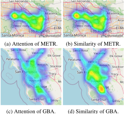
Pioneering works address above challenges from multiple perspectives. For scalability, there is a tendency to employ linear models, consisting of linear attentions [Liang et al., 2023] and MLP-Mixers [Zhang et al., 2023]. Among them, MLP-Mixers stand out for its lightweight and lower training costs. However, above efforts process all samples indiscriminately, introducing massive noise through global feature integration, which limits their effectiveness on large-scale data. To mitigate this, some approaches [Fang et al., 2024] group highly correlated samples into patches, enabling information exchange at the patch level. While this reduces computational complexity and partially addresses effectiveness, predefined patches fail to capture the evolving correlations of spatiotemporal data. Thus, developing a linear model that dynamically identifies key features is essential. Yet, explicitly defining key features is challenging, as they are shaped by complex and evolving spatiotemporal patterns.
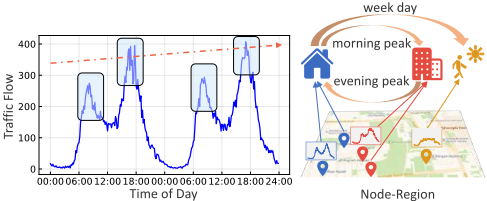
Fortunately, spatiotemporal data exhibit a hierarchical structure, which becomes more evident with increasing data scale. As illustrated in Figure 2, at the micro-level, local proximity prevails, with neighboring samples sharing similar values. At the macro-level, temporal data is driven by tendency and periodicity, while spatial data is influenced by semantic relevance. In summary, spatiotemporal data at different data resolutions exhibit distinct dominant patterns, generating specific key features. Such hierarchy is essential to address large-scale data problems, as these dominant patterns enable models to prioritize key samples, effectively filtering out irrelevant noise. Moreover, extracting key features at each individual data resolution is more effective and manageable than directly capturing global key features from the entire dataset. Motivated by the above analysis, we designed a linear model based on a hierarchical paradigm.
Technically, we proposed HieraMix, a Hierarchical SpatioTemporal Mixer model built entirely on Multi-Layer Perceptrons (MLPs). The core of HieraMix is the spatiotemporal mixing block, which hierarchically extracts and integrates spatiotemporal features. This block comprises a temporal aggregation mixer for temporal local features extraction and a spatial cascade mixer modeling hierarchical region-level spatial features. Furthermore, we design an adaptive region mixer that dynamically mixes features based on regional semantics. As a linear model, HieraMix is computationally efficient to large-scale datasets. By focusing on region-level dependencies, HieraMix reduces the noise introduced by global modeling. Our contributions are summarized as follows:
- We propose HieraMix for large-scale traffic prediction. The model generates hierarchical spatiotemporal features through bottom-up aggregation and integrates these features with a top-down propagation mechanism.
- We design an adaptive region mixer that generates transformation matrices based on regional semantics, enabling to dynamically model spatiotemporal patterns for different regions.
- Extensive experiments are conducted on four large-scale datasets, and HieraMix consistently outperforms stateof-the-arts, with average improvements of 5.32%, 3.64% and 3.55% in MAE, RMSE, and MAPE, respectively.
2 RelatedWork
Traffic Forecasting aims to predict traffic dynamics, e.g., traffic flow [Wang et al., 2022; Ji et al., 2023a; Ji et al., 2022], traffic speed [Liu et al., 2024b; Wang et al., 2016]. Early deep learning-based methods leverage Recurrent Neural Networks [Li et al., 2018; Bai et al., 2020] or Temporal Convolutional Networks [Wu et al., 2019] to capture temporal dependencies, while Graph Neural Networks are used to model spatial dependencies [Han et al., 2025; Ji et al., 2023b]. Transformer-based models are widely applied to various urban spatio-temporal tasks, such as trajectory representation [Jiang et al., 2023b; Yu et al., ], and general time-series forecasting [Wang et al., 2023; Wang et al., 2020]. Recently, they also gain considerable popularity in traffic forecasting [Jiang et al., 2023a; Ji et al., 2025; Deng et al., 2025]. However, the intensive convolution operations of GNNs [You et al., 2020] and the quadratic complexity of transformers limit their ability on large-scale urban.
Large-Scale Traffic Forecasting presents significant scalability challenges due to its extensive spatial scope, demanding models that are both efficient and effective. While some pioneering works reduce computational costs through graph decomposition [Fang et al., 2024; Wang et al., 2024b] or prior assumptions [Duan et al., 2024], they may compromise information integrity. More recently, researchers begin to employ MLP-Mixers for modeling large-scale data, owing to their effectiveness and scalability. MLPST [Zhang et al., 2023] first applies the MLP-Mixer architecture to grid-based data. TimeMixer [Wang et al., 2024a] performs node-level traffic forecasting by feature decomposition, but it lacks consideration of spatial correlations. TSMixer [Chen et al., 2023] and RPMixer [Yeh et al., 2024] mix temporal and spatial dimensions, effectively capturing spatiotemporal dependencies. Despite their efficiency, these methods indiscriminately construct global correlations across all data samples. When facing large-scale data, it will overwhelm key features with substantial irrelevant noise. Recent works [Wang et al., 2026] also highlight the importance of reducing noisy context.
3 Preliminary
Traffic Data. Traffic data consists of a series of numerical values collected and recorded by sensors in the urban traffic network. For the node n, xhn denotes traffic data at the h-th time slice. For a traffic network with N nodes, Xh ∈ RN denotes overall traffic data at the h-th time slice. Further, X t-T+1 : t denotes a traffic data series from t - T + 1 to t, where X t-T+1 : t = (Xt-T+1 , · · · ,Xt ) ∈ RN×T .
Traffic Forecasting. Given a traffic data series X t-T+1 : t with its next T ′ steps Y t+1:t+T ′ = X t+1:t+T ′ . The objective of traffic forecasting is to learn a function F that predicts the future traffic data:
where ˆ Y t+1 : t+T ′ is the prediction to Y t+1 : t+T ′ , and Θ denote the parameters to learn.
4 Methodology
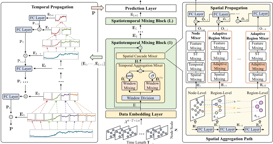
Based on above analysis, the primary motivation for largescale traffic forecasting is to leverage the hierarchy of spatiotemporal data. Therefore, we propose our HieraMix, a hierarchical MLP-Mixer model. As shown in Figure 3, our HieraMix consists of three parts. Details of each part are described in the following sections.
4.1 Data Embedding Layer
In the data embedding layer, raw traffic data is first transformed into high-dimensional embeddings and then integrated with the spatial and temporal embeddings.
The spatial embeddings reflect the correlations between nodes in the traffic network, comprising static and dynamic components. Specifically, the static component consists of node embeddings extracted from network topology through Node2Vec [Grover and Leskovec, 2016], denoted as Estatic ∈ RN×d , where d is the feature dimension. The dynamic component includes learnable vectors Edynamic ∈ RN×d to capture dynamic variations of each node. The overall spatial embeddings Esp ∈ RN×d are then obtained by:
The temporal embeddings complement periodic patterns for traffic data, including two temporal components: minuteof-day (1 to 60 × 24) embeddings Eday ∈ RT×d and day-ofweek (1 to 7) embeddings Eweek ∈ RT×d . Subsequently, the temporal embeddings Ete ∈ RT×d are computed as:
Overall, the raw traffic data X t-T+1:t is first transformed by a fully connected (FC) layer into Etr ∈ RN×T×d . Then, Etr incorporates Esp and Ete to generate the input embeddings E1 ∈ RN×T×d for subsequent ST mixing blocks:
4.2 Spatiotemporal Mixing Block
Motivation. Spatiotemporal data exhibits hierarchical characteristics, with dominated patterns vary with data resolutions. Our method aims to generate multi-resolution features through a bottom-up feature aggregation mechanism. The lower layers retain local characteristics, while the higher layers progressively incorporate global contextual features. This structured progression captures the transition between local and global properties and fully models patterns at different spatial scales. Specifically, we proposed the spatiotemporal mixing block (ST mixing block) based on the MLP-Mixer. By stacking multiple ST mixing blocks, hierarchical feature pyramids are generated efficiently.
Overall Structure. As shown in Figure 3, HieraMix consists of L spatiotemporal mixing blocks, each ST mixing block comprises two sequential modules: a temporal aggregation mixer and a spatial cascade mixer. The temporal mixer captures local temporal features and aggregates them to generate macro-level features, forming a temporal feature pyramid across ST mixing blocks. The spatial cascade mixer focuses on spatial hierarchies, employing a cascade of mixers to construct a spatial feature pyramid and capture spatiotemporal patterns at specific time scale within each ST mixing block. Stacking multiple ST mixing blocks produces spatiotemporal features at various resolutions, which are integrated to obtain the final spatiotemporal representation.
Supposed El ∈ RN×Tl-1×d denotes the input of the l-th
ST mixing block, where N is the number of nodes and Tl-1 is
the temporal length. Initially, the temporal aggregation mixer
takes El as input and outputs Hl. Then, Hl is processed by
the spatial cascade mixer.
Temporal Aggregation Mixer
Firstly, El is divided into multiple p-length windows, where
El ∈ RN×(Tl×p)×d , and Tl = ⌈Tl-1/p⌉ is the window size.
Each window is processed by a shared structure which com-
prises two parallel window mixing MLPs. Each MLP applies
two FC layers along the window-feature dimension (p × d).
For each window mixing MLP, El is aggregated as ˜El ∈
RN×Tl×h by the first FC layer, where h is the intermedi-
ate feature dimension. Further, the positional embedding
Epe ∈ RN×Tl×h is added to ˜El to identify the position in-
formation of each window. The second FC layer processes
˜El and outputs ˆHl ∈ RN×Tl×d :
ˆHl = FC2 (ϕ (FC1 (El) + Epe)) ,
(5)
where ϕ(·) is the activation function. Considering there are
two independent window mixing MLPs, let ˆH(1)
l and ˆH(2)
l
denote the output of these two MLPs respectively. To im-
prove the expressive power of the model, we employ the
gated mechanism [Dauphin et al., 2017] to generate the out-
put Hl ∈ RN×Tl×d of the temporal aggregation mixer.
Hl = tanh ( ˆH(1)
l
) ⊙ σ ( ˆH(2)
l
) ,
(6)
where tanh(·) represents the tanh function, σ(·) denotes the
sigmoid function, and ⊙ is dot-product.
Unlike typical Mixers that preserve the input's shape, our
temporal aggregation mixers integrate features within the
same window. When p is small, values within each window
exhibit gentle variations, dominated by the local similarity
characteristics. As a result, feature aggregation can effec-
tively capture local patterns and progressively adjust feature
scale by reducing the number of windows across ST mix-
ing blocks. For subsequent blocks, each window progres-
sively contains richer information and reveals macro-level
correlations like tendency. After the l-th layer, the input
El ∈ RN×(Tl×p)×d is aggregated as Hl ∈ RN×Tl×d .
Spatial Cascade Mixer
Overall Structure. Similar to temporal correlations, spatial correlations are also multi-scale. At the node-level, correlations are dominated by local similarity. While at the regionlevel, they depend on the scale and semantics of regions. Therefore, we designed the spatial cascade mixer, consisting of a spatial aggregation path, a node mixer and K adaptive region mixers corresponding to K region scales.
The spatial aggregation path consists of K FC layers. Given the dynamic nature of spatial correlations and the lack of predefined regions, Hl ∈ RN×Tl×d is first progressively aggregated into a set of region-level features across different scales through the aggregation path, represented as {Hl,1, · · · ,Hl,K}. Suppose Hl,k ∈ RSk×Tl×d is the input of the k-th adaptive region mixer, Sk is the amount of regions in this mixer, and (Sk+1 < Sk < · · · < S1 < N).
Subsequently, each mixer processes the input along spatial, temporal, and feature dimensions. The specific structure of each mixer is illustrated in Figure 3. Differed from the node mixer, the region mixer employs an adaptive mixing MLP to capture each region's unique features. As each region represents a distinct semantic unit, the adaptive mixing MLP ensures semantically similar regions share similar parameters, and vice versa. Each mixer generates its individual output, and the final output integrates features from both node-level and multiple region-level features.
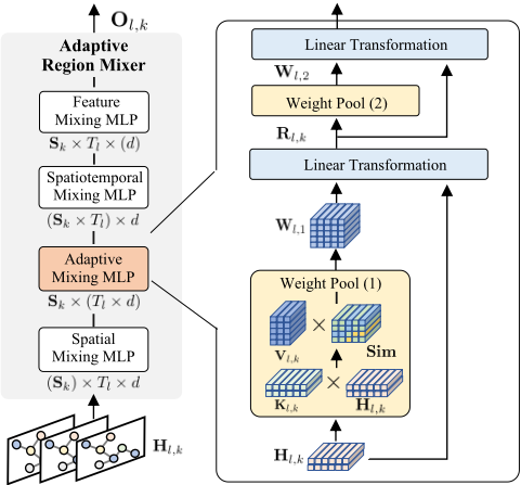
Adaptive Region Mixer. As shown in Figure 4, the k-th adaptive region mixer processes Hl,k ∈ RSk×Tl×d through four MLPs: the spatial mixing MLP, the adaptive mixing MLP, the spatiotemporal mixing MLP, and the feature mixing MLP to capture spatiotemporal dependencies at the corresponding scale. Notably, the adaptive mixing MLP is different as it employs a parameter pool to adaptively generate transformation matrices tailored to each region's semantics.
Specifically, the parameter pool contains Kl,k ∈ RMk×Tl as keys and Vl,k ∈ RMk×Tl×h as base weights, where h is the intermediate feature dimension and Mk is the size of base weights. Then, the demanding parametersWl,k ∈ RSk×Tl×h are generated as follows:
where ∗ denotes the matrix multiplication, Sim ∈
RSk×d×Mk are weight scores, and Sim(i) is the i-th tensor of Sim over the feature dimension (d).
In the adaptive mixing MLP, both two FC layers are generated from the parameter pool, denoted as Wl,k,1 and Wl,k,2. Then, the input Hl,k is transformed as:
where H(j) l,k , W(j) l,k,1 are both the j-th tensor over the spatial dimension, and Rl,k ∈ RSk×d×h denotes the hidden state.
To increase the semantic distinctiveness of each region, we employ the parameter orthogonal loss (POL) during training. It minimizes the similarity between each W(i) l,k and W(j) l,k to decrease the semantic similarity among regions. Specifically, the POL in the l-th ST mixing block can be formalized as:
where CS(·) represents the cosine similarity. The total orthogonal loss can be denoted as:
Output. The spatial cascade mixer generates an output set, including {Ol,g,Ol,1, · · · ,Ol,K}, where Ol,g ∈ RN×Tl×d belongs to the node mixer, and Ol,k ∈ RSk×Tl×d belongs to the k-th adaptive region mixer.
Hierarchical Feature Propagation
Since HieraMix processes spatiotemporal data hierarchically, it generates various feature pyramids: (1) Stacked ST mixing blocks form a feature pyramid across temporal resolutions, and the higher features reflect the trend of the lower features. (2) In each ST mixing block, the spatial cascade mixer generates a feature pyramid across spatial resolutions, and the higher regions reflect the interactions between lower nodes. Therefore, the hierarchical feature propagation is proposed for feature integration. It contains two top-down paths: the spatial propagation and the temporal propagation.
Spatial Propagation. The top-down spatial feature propagation starts with the output Ol,K. It is transformed by an FC layer into ˆOl,K ∈ RSk-1×Tl×d . As shown in Figure 3, Ol,k is transformed into ˆOl,k as follows:
where El+1 denotes the final result of the spatial propagation, which serves as the input of the (l + 1)-th ST mixing block.
Temporal Propagation. Stacked ST mixing blocks will generate a feature pyramid across temporal resolutions, denoted as {E1, · · · ,El, · · · ,EL+1}. Additionally, EL+1 is the output of the L-th ST mixing block. Similar as the spatial propagation, temporal propagation begins with EL+1, which is first projected by an FC layer into PL+1. As shown in Figure 3, El is transformed into Pl ∈ RN×Tl×d as follows:
where P ∈ RN×T×d denotes the final result.
| Datasets | Nodes | Time steps | Time Range |
|---|---|---|---|
| SD | 716 | 35040 | 1/1/2019-1/1/2020 |
| GBA | 2352 | 35040 | 1/1/2019-1/1/2020 |
| GLA | 3834 | 35040 | 1/1/2019-1/1/2020 |
| CA | 8600 | 35040 | 1/1/2019-1/1/2020 |
4.3 Prediction Layer
The prediction layer, takes P ∈ RN×T×d and EL+1 ∈ RN×TL×d as inputs and regresses the prediction values as:
To optimize the model, we employ the mean absolute error (MAE) as the regression loss, which is denoted as LREG. The overall loss combines the regression loss and the parameter orthogonal loss, which can be formalized as L:
where α and β are hyper-parameters for weight balance.
5 Experiments
5.1 Experiment Setup
Datasets. We evaluate HieraMix on four datasets within LargeST [Liu et al., 2024a], including SD, GBA, GLA, and CA. Details of each dataset are described in Table 1. Following previous works, we aggregate the time intervals from 5-minutes into 15-minutes. We divide each dataset according to four seasons, and then splite the training, validation and test sets with the ratio of 6:2:2 in each season.
Baselines. The HieraMix is compared with 20 baseline models, including 11 Previous SOTAs and 9 Scalable Models for Large-Scale Settings.
Experiment Details. All experiments are conducted on Ubuntu 20.04.6 LTS with an NVIDIA RTX A6000 48GB GPU, based on the LibCity [Wang et al., 2021]. Our HieraMix takes 12 historical time slices as input to predict the next 12 time slices. We use the mean absolute error (MAE), the root mean square error (RMSE) and the mean absolute percentage error (MAPE) as evaluation metrics.
5.2 Performance Comparisons
Table. 2 presents the overall performance of our model and all the baselines with respect to MAE, RMSE, and MAPE on four datasets. Additionally, we run all models five times and report the mean results. Overall, HieraMix consistently outperforms other baselines on all four datasets. Specifically, HieraMix obtains average improvements of 5.32%, 3.64% and 3.55% beyond the best baselines in MAE, RMSE and MAPE, respectively. Furthermore, based on the experimental results, we can make the following observations:
Hierarchical Processing Benefits Performance. In most cases, the performance of scalable baselines is much inferior to previous transformer-based models. However, HieraMix enables a linear MLP-Mixer model to outperform complex transformer-based baselines across all four datasets. This is due to hierarchical processing, which allows the model to learn dominant features at different scales, generating more effective representations.
| Model | SD | GBA | GLA | CA | ||||||||
|---|---|---|---|---|---|---|---|---|---|---|---|---|
| MAE | RMSE | MAPE | MAE | RMSE | MAPE | MAE | RMSE | MAPE | MAE | RMSE | MAPE | |
| DCRNN [Li et al., 2018] | 17.96 | 28.65 | 11.85 | 21.86 | 34.65 | 20.19 | 23.36 | 36.19 | 14.19 | 28.24 | 44.01 | 22.23 |
| STGCN [Yu et al., 2018] | 16.87 | 28.84 | 9.76 | 19.96 | 32.78 | 16.27 | 18.61 | 30.18 | 11.44 | 17.87 | 29.14 | 13.56 |
| ASTGCN [Guo et al., 2019] | 19.99 | 32.19 | 12.99 | 22.97 | 36.35 | 20.39 | 21.46 | 34.21 | 13.29 | - | - | - |
| GWNET [Wu et al., 2019] | 16.93 | 27.97 | 9.74 | 19.73 | 31.99 | 17.54 | 18.94 | 30.16 | 11.58 | 19.73 | 31.32 | 15.42 |
| STGODE [Fang et al., 2021] | 17.55 | 28.67 | 11.25 | 19.73 | 32.45 | 16.28 | 18.86 | 30.49 | 11.81 | 17.76 | 29.13 | 13.37 |
| DSTAGNN [Lan et al., 2022] | 17.37 | 27.68 | 11.27 | 20.14 | 32.63 | 16.37 | 18.62 | 30.00 | 11.20 | - | - | - |
| D2STGNN [Shao et al., 2022b] | 16.49 | 26.59 | 9.62 | 18.56 | 31.12 | 13.05 | - | - | - | - | - | - |
| HIEST [Ma et al., 2023] | 17.94 | 29.03 | 10.33 | 22.50 | 35.75 | 14.02 | 22.37 | 35.26 | 11.84 | 22.06 | 35.03 | 14.18 |
| PDFormer [Jiang et al., 2023a] | 15.84 | 25.91 | 9.70 | - | - | - | - | - | - | - | - | - |
| DGCRN [Li et al., 2023] | 15.60 | 25.90 | 9.93 | 19.11 | 31.21 | 14.17 | - | - | - | - | - | - |
| TESTAM [Lee and Ko, 2024] | 18.51 | 30.42 | 10.42 | 19.57 | 32.32 | 13.94 | - | - | - | - | - | - |
| STID [Shao et al., 2022a] | 18.21 | 29.97 | 10.18 | 20.82 | 34.43 | 13.19 | 19.83 | 32.33 | 10.38 | 19.11 | 31.45 | 11.68 |
| FreTS [Yi et al., 2023] | 23.95 | 37.12 | 14.89 | 26.87 | 40.55 | 18.39 | 27.76 | 42.00 | 15.85 | 27.58 | 42.50 | 18.47 |
| TSMixer [Chen et al., 2023] | 16.81 | 29.79 | 10.52 | 19.93 | 34.83 | 16.56 | 17.86 | 30.89 | 10.96 | 16.78 | 29.42 | 12.43 |
| TimeMixer [Wang et al., 2024a] | 17.15 | 28.30 | 9.74 | 21.74 | 35.15 | 13.85 | 19.76 | 31.96 | 10.81 | 18.16 | 30.11 | 11.61 |
| RPMixer [Yeh et al., 2024] | 16.72 | 29.64 | 10.63 | 19.05 | 32.75 | 15.26 | 17.57 | 30.42 | 10.56 | 16.75 | 29.28 | 12.36 |
| PatchSTG [Fang et al., 2024] | 15.93 | 28.19 | 9.69 | 18.94 | 33.02 | 13.17 | 17.53 | 29.72 | 10.02 | 16.69 | 28.58 | 11.50 |
| EiFormer [Sun et al., 2025] | 17.90 | 32.06 | 10.79 | 20.39 | 35.35 | 15.58 | 18.91 | 33.05 | 11.00 | 18.22 | 32.07 | 12.89 |
| GSNet [Kong et al., 2025] | 16.65 | 27.33 | 9.62 | 19.37 | 31.98 | 13.15 | 18.81 | 30.65 | 10.09 | 17.61 | 29.15 | 11.15 |
| LSTNN [Wang et al., 2025] | 15.83 | 27.08 | 9.59 | 18.48 | 31.59 | 13.11 | 17.48 | 29.71 | 9.95 | 16.58 | 28.24 | 11.05 |
| HieraMix | 14.80 | 25.06 | 9.22 | 17.73 | 30.67 | 12.71 | 16.45 | 28.03 | 9.53 | 15.55 | 27.05 | 10.55 |
Advantages of Scalability. The experiments validate the scalability challenges inherent in previous SOTAs. Several GNN- and transformer-based models are unable to complete the experiments on larger datasets due to prohibitive computational and memory costs. In contrast, HieraMix demonstrates excellent scalability, efficiently handling all datasets.
Advantages of Robustness. The performance gap between HieraMix and the second-best baseline widens with larger datasets. On the smallest dataset, HieraMix outperforms the second-best baseline by 2.85% in MAPE. On the largest dataset, this gap increases to 4.52% in MAPE. This demonstrates HieraMix's robustness with large-scale datasets.
5.3 Ablation Study
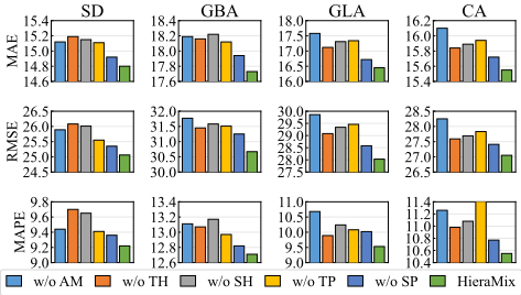
We conduct ablation studies to analyze the effectiveness of each component in HieraMix. These five variants are listed as below: (1) w/o AM: Replaces the adaptive mixing MLP with a standard mixing MLP. (2) w/o TH: Removes the modeling of temporal hierarchy, i.e., the time length in each ST mixing block remains the same. (3) w/o SH: Removes the modeling of spatial hierarchy, i.e., the number of nodes in the spatial cascade mixer remains the same. (4) w/o TP: Removes the temporal propagation. (5) w/o SP: Removes the spatial propagation. Ablation results are shown in Figure 5, which can be concluded as:
Benefits Brought by Hierarchical Modeling. w/o SH and w/o TH are both inferior to HieraMix, which demonstrates the effectiveness of hierarchical modeling in both spatial and temporal dimensions. Additionally, HieraMix performs better than w/o AM, because adaptive mixing improves semantic differences between regions, resulting in more structured hierarchical features.
Effectiveness of Feature Propagation. As HieraMix outperforms w/o TP and w/o SP, it indicates that features at different scales contain distinct semantic information. The feature propagation enables multi-scale features to complement each other, providing more comprehensive representations.
5.4 Efficiency Analysis
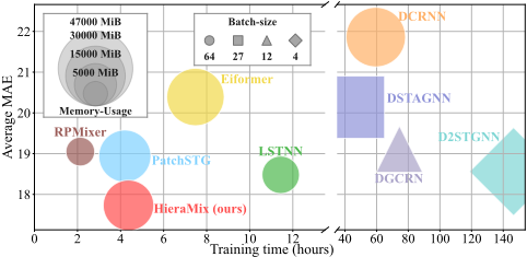
In this section, we evaluate HieraMix and baselines in terms of performance and efficiency, and present results on MAE and the total training time on the GBA dataset. As shown in Figure 6, HieraMix significantly outperforms linear baselines and even surpasses SOTA transformer-based models (e.g., PatchSTG, Eiformer). Meanwhile, HieraMix maintains efficiency comparable to mainstream scalable models (e.g., RPMixer, LSTNN). This demonstrates that HieraMix balances performance and efficiency, offering excellent scalability on large-scale datasets.
Further, we analyze the computational cost of HieraMix. Specifically, the mixing operation mainly consists of two linear transformations with a time complexity of O(dhNT). Generating adaptive transformation weights incurs a complexity of O(MdhNT ), and applying these weights for linear transformations adds another O(dhNT). Consequently, the total complexity is O(LKMdhNT), where L and K represent the number of ST mixing blocks and region scales, respectively. This linear complexity with respect to N ensures scalability for large-scale spatiotemporal prediction.
5.5 Parameter Sensitivity
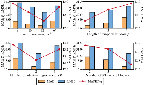
We analyze the impact of four key hyperparameters in the GBA dataset. The results are illustrated in Figure 7.
Size of base weights M. The adaptive mixing MLP generates region-specific matrices over a parameter pool with M sets base weights. Smaller M strengthens parameter sharing but limits adaptivity, while larger M enriches the basis components for composition. However, overly large parameter pool can increase optimization difficulty and impair the model's generalization ability.
Length of temporal window p. The temporal aggregation mixer partitions the sequence into non-overlapping windows
- (a) Visualization of HieraMix.
- (b) Visualization of w/o AM.
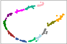
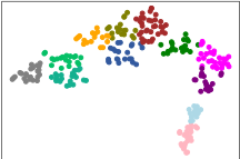
Figure 8: t-SNE of OL,1 of HieraMix and w/o AM on GBA. Each color denotes a region-type cluster in the embedding space.
of length p and performs within-window aggregation. Figure 7 shows a clear degradation as p increases. This behavior is consistent with the design motivation that local temporal proximity exhibits strong similarity, which can be effectively captured when p is small. A larger p may over-smooth shortterm variations and discard high-frequency signals that are crucial for short-horizon prediction.
Number of adaptive region mixers K. This determines the number of region scales in the spatial cascade mixer and controls the depth of spatial hierarchy. Moderate K supports multi-scale regional semantics. When K is small, the spatial hierarchy becomes insufficient, limiting ability to capture multi-scale regional semantics simultaneously. Excessively large K introduces additional coarser aggregation levels that may inject extra noise.
Number of STmixing blocks L. This controls the depth of hierarchical spatiotemporal mixing and the resulting feature pyramids. Increasing L expands the temporal receptive field, enabling higher layers to capture broader trends and to refine lower-level representations through top-down propagation.
5.6 Visualization
To evaluate HieraMix's ability to capture regional semantics, we leverage t-SNE to visualize the spatial representations OL,1 produced by the HieraMix and its w/o AM variant. As illustrated in Figure 8, the representations generated by HieraMix are more compact with well-defined boundaries between clusters. In contrast, the w/o AM variant yields representations with substantial overlap between clusters. This comparison highlights HieraMix's greater representation ability, which ensures nodes within the same region type share similar spatiotemporal patterns, while nodes across different types maintain distinct characteristics.
6 Conclusion
We present HieraMix, a simple yet effective MLP-Mixer model, which leverages hierarchical modeling to tackle large-scale traffic forecasting. HieraMix surpasses all current baselines and introduces enhancements to the MLPMixer architecture, making it competitive with more complex transformer-based models. Comprehensive experiments on extensive traffic datasets demonstrate its scalability and effectiveness. Future work will extend its application to multivariate time series prediction and anomaly detection.
Acknowledgments
This work is supported by the National Natural Science Foundation of China (No. 725B2004, 72242101, 72222022, 72171013), State Key Laboratory of Complex & Critical Software Environment (SKLCCSE-2025ZX-17), and the Special Fund for Health Development Research of Beijing (2024-2G-30121).
Contribution Statement
† Yongyao Wang and Xie Yu contributed equally to this work.
@inproceedings{ijcai2026p729,
  title     = {HieraMix: A Hierarchical MLP-Mixer for Large-Scale Traffic Forecasting},
  author    = {Wang, Yongyao and Yu, Xie and Wang, Jingyuan and Ji, Jiahao and Chao, Li},
  booktitle = {Proceedings of the Thirty-Fifth International Joint Conference on
               Artificial Intelligence, {IJCAI-26}},
  publisher = {International Joint Conferences on Artificial Intelligence Organization},
  editor    = {Diego Calvanese},
  pages     = {6555--6563},
  year      = {2026},
  month     = {8},
  note      = {AI4Tech: AI Enabling Technologies},
  doi       = {10.24963/ijcai.2026/729},
  url       = {https://doi.org/10.24963/ijcai.2026/729},
}
TY - CPAPER TI - HieraMix: A Hierarchical MLP-Mixer for Large-Scale Traffic Forecasting AU - Wang, Yongyao AU - Yu, Xie AU - Wang, Jingyuan AU - Ji, Jiahao AU - Chao, Li T2 - Proceedings of the Thirty-Fifth International Joint Conference on Artificial Intelligence, IJCAI-26 PB - International Joint Conferences on Artificial Intelligence Organization PY - 2026 SP - 6555 EP - 6563 DO - 10.24963/ijcai.2026/729 UR - https://doi.org/10.24963/ijcai.2026/729 ER -Copied
Machine-readable versions of this paper, for tools and AI agents:





