
When Do GNNs Work: Understanding and Improving Neighborhood Aggregation
Proceedings of the Twenty-Ninth International Joint Conference on Artificial Intelligence. Main track. Pages 1303-1309.
https://doi.org/10.24963/ijcai.2020/181
Keywords
- Data Mining: Mining Graphs, Semi Structured Data, Complex Data
- Machine Learning: Semi-Supervised Learning
Abstract
Graph Neural Networks (GNNs) have been shown to be powerful in a wide range of graph-related tasks. While there exists various GNN models, a critical common ingredient is neighborhood aggregation, where the embedding of each node is updated by referring to the embedding of its neighbors. This paper aims to provide a better understanding of this mechanisms by asking the following question: Is neighborhood aggregation always necessary and beneficial? In short, the answer is no. We carve out two conditions under which neighborhood aggregation is not helpful: (1) when a node's neighbors are highly dissimilar and (2) when a node's embedding is already similar with that of its neighbors. We propose novel metrics that quantitatively measure these two circumstances and integrate them into an Adaptive-layer module. Our experiments show that allowing for node-specific aggregation degrees have significant advantage over current GNNs.
- [Chen et al., 2020] Deli Chen, Yankai Lin, Wei Li, Peng Li, Jie Zhou, and Xu Sun. Measuring and relieving the over- smoothing problem for graph neural networks from the topological view. AAAI, 2020.
- [Hamilton et al., 2017] William L. Hamilton, Zhitao Ying, and Jure Leskovec. Inductive representation learning on large graphs. In NIPS, 2017.
- [Hou et al., 2020] Yifan Hou, Jian Zhang, James Cheng, Kaili Ma, Richard T. B. Ma, Hongzhi Chen, and Ming- Chang Yang. Measuring and improving the use of graph information in graph neural networks. In ICLR, 2020.
- [Kipf and Welling, 2016] Thomas Kipf and Max Welling. Semi-supervised classification with graph convolutional networks. ICLR, 2016.
- [Klicpera et al., 2019] Johannes Klicpera, Aleksandar Bo- jchevski, and Stephan Günnemann. Combining neural networks with personalized pagerank for classification on graphs. In ICLR, 2019.
- [Li et al., 2018] Qimai Li, Zhichao Han, and Xiao-Ming Wu. Deeper insights into graph convolutional networks for semi-supervised learning. In AAAI, 2018.
- [Namata et al., 2012] Galileo Mark Namata, Ben London, Lise Getoor, and Bert Huang. Query-driven active survey- ing for collective classification. In Workshop on Mining and Learning with Graphs, 2012.
- [Perozzi et al., 2014] Bryan Perozzi, Rami Al-Rfou, and Steven Skiena. Deepwalk: online learning of social rep- resentations. KDD, 2014.
- [Sen et al., 2008] Prithviraj Sen, Galileo Namata, Mustafa Bilgic, Lise Getoor, Brian Gallagher, and Tina Eliassi- Rad. Collective classification in network data. In AI mag- azine, 2008.
- [Velickovic et al., 2017] Petar Velickovic, Guillem Cucurull, Arantxa Casanova, Adriana Romero, Pietro Liò, and Yoshua Bengio. Graph attention networks. ICLR, 2017.
- [Wang et al., 2019] Minjie Wang, Lingfan Yu, Da Zheng, Quan Gan, Yu Gai, Zihao Ye, Mufei Li, Jinjing Zhou, Qi Huang, Chao Ma, Ziyue Huang, Qipeng Guo, Hao Zhang, Haibin Lin, Junbo Zhao, Jinyang Li, Alexander Smola, and Zheng Zhang. Deep graph library: Towards efficient and scalable deep learning on graphs, 2019.
- [Wu et al., 2012] Xiaoming Wu, Zhenguo Li, Anthony M. So, John Wright, and Shihfu Chang. Learning with par- tially absorbing random walks. In NIPS, pages 3077-3085. 2012.
- [Wu et al., 2019] Felix Wu, Tianyi Zhang, Amauri H. de Souza, Christopher Fifty, Tao Yu, and Kilian Q. Wein- berger. Simplifying graph convolutional networks. In ICML, 2019.
- [Yang et al., 2016] Zhilin Yang, William W. Cohen, and Ruslan Salakhutdinov. Revisiting semi-supervised learn- ing with graph embeddings. In ICML, 2016.
- [Zachary, 1977] Wayne W. Zachary. An information flow model for conflict and fission in small groups. 1977.
- [Zhang and Meng, 2020] Jiawei Zhang and Lin Meng. Gres- net: Graph residual network for reviving deep gnns from suspended animation, 2020.
- [Zhao and Akoglu, 2020] Lingxiao Zhao and Leman Akoglu. Pairnorm: Tackling oversmoothing in gnns. In ICLR, 2020.
- [Zhou et al., 2018] Jie Zhou, Ganqu Cui, Zhengyan Zhang, Cheng Yang, Zhiyuan Liu, and Maosong Sun. Graph neural networks: A review of methods and applications. ArXiv, abs/1812.08434, 2018.
References were extracted automatically from the PDF and may contain errors.
Full text extracted automatically from the PDF; figures, tables and equations may differ. The PDF is the version of record.
1 Introduction
Graph neural networks (GNNs) are a class of neural network models for graphs which learn to integrate node features based on labels and link structures [Zhou et al., 2018]. Despite the impressive performance, the structure of a typical GNN model, i.e., a graph convolutional network (GCN) [Kipf and Welling, 2016], is quite simple. It can be regarded as a fully-connected neural network (FNN) plus a neighborhood aggregation component. The former computes a nonlinear feature projection, whereas the latter mixes the feature of each node with those of its neighbors, allowing the model to leverage graph topology for feature learning.
Despite the great success of GNN in several datasets, we observe that in some cases the improvement over a simple FNN that has no access to links in the graph is limited, especially when the aggregation degree (i.e., rounds of aggregation) is large (Table 1). This leads us to question whether neighborhood aggregation may be harmful or unnecessary in certain cases. Existing studies have looked into this from a global perspective. They observe that high aggregation degrees over the entire graph mixes together nodes from different clusters, and name this phenomenon as 'over-smoothing' [Li et al., 2018; Chen et al., 2020; Zhao and Akoglu, 2020; Hou et al., 2020]. However, none of them has considered different aggregation degrees from a local perspective. In fact, if we allow the aggregation degrees to vary across nodes, the performance of GNN can be significantly improved (as shown in the last row of Table 1). The next question is how can we control the aggregation degree for individual nodes?
∗Equal Contribution.
| Method | Aggregation degrees | Acc | |||
|---|---|---|---|---|---|
| 0 | 1 | 2 | ≥ 3 | ||
| FNN | 100% | 0 | 0 | 0 | 40.5% |
| 7-layer GNN | 0 | 0 | 0 | 100% | 40.8% |
| 2-layer GNN | 0 | 0 | 100% | 0 | 77.1% |
| Node-wise Agg | 7.4% | 1.1% | 83.2% | 8.3% | 86.8% |
Towards this goal, we try to characterize cases where aggregation is not helpful. Specifically, for an individual node, we analyze the utility of neighborhood aggregation based on the features/predicted labels of itself and its immediate neighbors. We find that: (1) If the learned feature/label of a center node's neighbors disagree (have high entropy), further aggregation may hurt performance; (2) When the learned feature/label of a center node is nearly identical to its neighbors, further aggregation is unnecessary. For each of the scenarios, we design an intuitive and principled metric based on information theory to quantify its presence.
To make use of our metrics and realize the full potential of GNNs, we design an Adaptive-layer module that allows individual nodes to perform different rounds of neighborhood aggregation. Specifically, during the training process, we check each node and their neighbors' learned label, estimate whether neighborhood aggregation is harmful or unnecessary by calculating our metrics, and only allow nodes where aggregation is useful to perform aggregation. We keep conducting this check-aggregate process until a certain number of iterations have been executed, or all nodes are not allowed to perform aggregation. Our module can be implemented efficiently and has similar runtime to GCN. We also provide extensive experiments and case studies to validate and explain the advantages of our proposed module.
To sum up, our key contributions are: (1) Analyzing the utility of neighborhood aggregation from a local perspective, with illustrative examples, theoretical support and empirical results; (2) Proposing two intuitive and principled metrics to quantitatively describe two scenarios where neighborhood aggregation is not helpful; (3) Incorporating the metrics into the design of a novel Adaptive-layer module, whose performance is validated through extensive experiments on three real-world networks.
2 Preliminary
GNN models have been intensively studied and applied to various graph-related tasks. In this work, we focus on semisupervised node classification [Kipf and Welling, 2016; Hamilton et al., 2017; Velickovic et al., 2017; Li et al., 2018; Chen et al., 2020; Zhang and Meng, 2020].
2.1 Graph Neural Networks (GNN)
Given a graph G = (V, E) with input features X, the update function of GNN for a single layer is as follows:
When the end task is node classification, another linear layer is used to project the node embedding to class labels:
We refer to the operation Agg({hlu |u ∈ N(v)}) as neighborhood aggregation since it essentially combines information from a node's neighborhood. The exact aggregation function and the definition of 'neighborhood' differs from model to model [Zhou et al., 2018]. In particular, GCN [Kipf and Welling, 2016] sums up the information from direct neighbors by defining
Since the aggregation-based update is done for each layer, we refer to the total number of layers L as aggregation degree.
2.2 Simple Graph Convolution (SGC)
SGC [Wu et al., 2019] simplifies GCN by removing the nonlinearity between layers. SGC has been shown to have similar performance as GCN with improved efficiency. Another benefit of using a single linear projection is that the number of parameters in SGC does not grow with the number of layers, sidestepping the over-fitting phenomenon. The resulting model can be expressed as follows:
where A is the adjacency matrix, ˜ A = A + I and ˜D is the degree matrix of ˜ A.
3 Analysis
In this section, we start from a case study to explore under which circumstances neighborhood aggregation may not be helpful to GNNs. The GNN update function consists of several operations, namely the non-linearity, linear projection and neighborhood aggregation. To avoid confounding factors such as overfitting, we use SGC [Wu et al., 2019] as our base model for investigation.
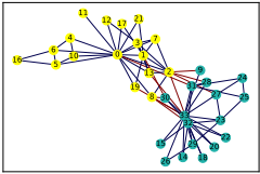
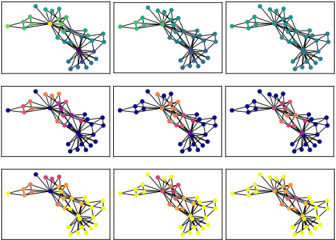
Zachary's karate club [Zachary, 1977] (Figure 1) is a classical dataset showing the interactions among club members. The club is divided into two groups, as shown by the yellow and blue nodes. We start with gradually increasing the aggregation degree L = 1, 3, 5 for SGC on this dataset to observe how the information propagates over the aggregation rounds (first row in Figure 2). When L = 1, the initial labeled nodes clearly stand out and information is only propagated to its direct neighbors and not sufficiently spread among all club members. When L = 3 the prediction among the same club is very similar but the inter-club distinction is still evident. As L continues to increase (L = 5 and over), the inter-club distinction begins to blur and finally all nodes have the same prediction. This phenomenon was referred to as over-smoothing in [Li et al., 2018]. In this example, to achieve the best classification results, we need neighborhood aggregation, but must retreat from excessive aggregation. The key to avoiding deterioration is to prevent inter-club, or more generally, inter-community mixing, which happens when the aggregation crosses the community boundary (nodes 13, 19, 1, 2). A major characteristic of these nodes is that its neighbors take on different labels, leading us to develop our first metric neighborhood entropy. Moreover, the best aggregation degree differs from node to node: when L = 1 bottom right group (nodes 32, 33, 14, 29) already produces the right prediction confidently, whereas nodes in the top (nodes 0, 11, 12, 17) still require more aggregation. For these confident nodes, further aggregation only increases computation cost, but does not contribute to performance. Thus, we derive our second metric center-neighbor similarity.
3.1 Neighborhood Entropy
Neighborhood aggregation takes advantage of the homophily effect in networks, which states that connected nodes should be similar. Taking this one step further, the neighbors of a node should be similar among themselves. When the neighbors disagree, we take this as a warning that the assumption may not hold and the aggregated information may be noise.
To measure the diversity of a particular node's neighborhood, we compute the entropy among neighbors:
where X is the feature space, f N(u) is the probability density function (PDF) of the features of node u's neighbors. However, since this PDF is a sum of Dirac functions at each neighbor over high dimensional space, computing this differential entropy is infeasible and also not very informative. Alternatively, we use the predicted labels to calculate the label distribution of node u's neighbors and calculate its discrete entropy:
where C is the set of all label classes. If Scoreetp(u) is larger, the diversity of node u's neighbor is larger. For the karate club dataset shown in Figure 1, when labels are correctly predicted, we have Scoreetp(9) = 0.673, which is much larger than Scoreetp(6) = 0, indicating that node 9's neighbors are more diverse than node 6's.
3.2 Center-Neighbor Similarity
Towards the other end of the spectrum, neighborhood aggregation may be redundant when a node's features are sufficiently similar to its neighbors. For example, the label of node 25 in Figure 2 is already the same as all of its neighbors when L = 1, so the aggregation operation will not change its label and is unnecessary.
We characterize this similarity by calculating the pointwise mutual information (PMI) between the center node and its neighbors' features: PMI(u;N(u)) = P(N(u)|u) P(N(u)) . Since we do not have prior knowledge of the probability distribution of the neighbors' features, we assume it follows the uniform distribution, which makes P(N(u)) a constant. The similarity is then defined as follows:
where u is the center node, N(u) is the neighbor set of u and fu is the node feature of u, which may be the input feature, the learned embedding, or the predicted label of the node. Similarly, we can use the one-hot predicted label to calculate the metric:
If Scoresim(u) is larger, node u is more similar to its neighbors. In this scenario, we can compare the performance before and after neighborhood aggregation and show that the prediction results are nearly the same, as formally induced in the following Theorem 1.
Theorem1. Assume we use hu, the predicted probability distribution for each label to calculate Scoresim. If we have Scoresim(u) ≥ ϵ for all u ∈ V , then the difference in 2norm loss in terms of before and after neighborhood aggregation ∆L ≤ √2(1 - ϵ|V | |C| ).
Proof. Let fu be the original feature of node u, lu be the onehot true label vector of u and hu be the original predicted label distribution. The predicted label distribution of node u after aggregation is ˆ hu = 1 |N (u)+1| ∑v∈N (u) ⋃{u} hv .
3.3 PuttingMetrics to Test
In the previous sections, we described the motivation and theoretical analysis behind our two proposed metrics neighborhood entropy and center-neighbor similarity. When either neighborhood entropy or center-neighbor similarity is high, we should be more cautious in performing aggregation.
Now we put our proposed metrics to test as shown in the second and third rows of Figure 2. The computed neighborhood entropy is shown in the second row, with deeper colors showing lower entropy. As seen from left to right, the high entropy nodes gradually shift from the top to the middle and converge at the nodes that should act as 'gatekeepers'
between communities. The third row shows the computed values of center-neighbor similarity. The bottom right group has high similarity after 1 round of aggregation and remains so throughout the process. As a comparison, the nodes on the top initially have low similarity with their neighbors, indicating that more aggregation is needed. At a first glance, the two rows may seem to be exactly opposite of each other and the two metrics are indeed designed to handle cases at two ends of the spectrum. The nodes that benefit from further aggregation are the ones that fall into neither of the categories and should have low values for both neighborhood entropy and center-neighbor similarity. By overlaying the two rows, we can see that the nodes that fall in this category gradually disappear with the increase of aggregation degree L, indicating that no more aggregation should be done.
4 Model
Following previous analysis, we propose an Adaptive-layer module, which allows nodes to make individual decisions at each round of neighborhood aggregation. As a result, different nodes may experience different aggregation degrees.
Specifically, in each layer, we apply a gating function that controls the influence of neighborhood information. Its value is determined by Scoresim and Scoreetp. We remove all non-linearities between layers in a similar spirit to SGC. The structure of our module is as follows:
where zl,u is a random variable controlling the usage of neighborhood aggregation. Our update function resembles a residual layer. There are two considerations in this design: (1) residual layers are known to allow the stacking of more layers and (2) we are able to project the hidden state hlu to labels at every layer with the same projection matrix Wy.
The gate zl,u is computed from Scoresim and Scoreetp using the following formula:
The activation function σ squeezes the value of z to (0, 1).
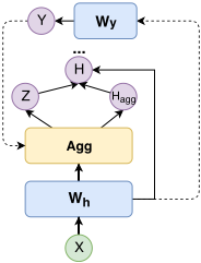
When either of Scoresim or Scoreetp is large, z takes on a small value close to 0. Norm is the batch normalization operation to rescale the scores so that they are comparable across layers.
For simplicity, we use the one-hot predicted label to calculate Scoresim and Scoreetp in our model. Since we do not have prior knowledge of the actual class size in practice, we assume all the label classes have the same size. So the label class size term is a constant and is left out from calculation.
To compare with attention based models, we can extend our base model to handle attention weights over neighbors:
where alu,v is the attention coefficient of node v for node u in the lth layer, which can be computed similarly to [Velickovic et al., 2017]. We can also extend our metrics to multihead attention by computing a different z for each attention head, denoted as zk l,u :
5 Experiments
In this section we conduct extensive experiments to test our module on the node classification problem. We refer to our base model as ALaGCN and our attention-enhanced model as ALaGAT.
5.1 Experiment Setup
Datasets. We conduct the experiments on three citation networks: Cora, CiteSeer [Sen et al., 2008] and PubMed [Namata et al., 2012]. The details are listed in Table 2. We tested with 1%, 3% and 5% training size for Cora and CiteSeer, and with 0.3%, 0.15% and 0.05% training size for PubMed. There rates are chosen for comparison with [Kipf and Welling, 2016] and other methods. We also run the experiments with the standard 20 labeled nodes per class setting to compare with reported performance.
| Datasets | Nodes | Edges | Classes | Features |
| Cora | 2708 | 5429 | 7 | 1433 |
|---|---|---|---|---|
| CiteSeer | 3327 | 4732 | 6 | 3703 |
| PubMed | 19717 | 44338 | 3 | 500 |
| Methods | Cora | CiteSeer | PubMed | ||||||
|---|---|---|---|---|---|---|---|---|---|
| 1% | 3% | 5% | 1% | 3% | 5% | 0.05% | 0.15% | 0.3% | |
| CS-GNN | 48.4 ± 3.4 (2) | 62.2± 4.0 (2) | 62.0 ± 6.5(2) | 45.1 ± 4.0 (2) | 56.4± 1.5 (2) | 60.5 ± 3.9 (2) | 60.5 ± 4.4 (2) | 68.4± 6.3 (2) | 74.0± 0.8 (2) |
| GResNet | 64.7 ± 3.7 (7) | 76.7 ± 2.2 (5) | 79.2 ±1.1(5) | 53.7 ± 3.6 (6) | 63.2± 2.5 (6) | 66.0 ± 0.5(4) | 66.2 ± 5.7 (7) | 75.0± 6.4 (7) | 79.5±2.0 (7) |
| Co/self-train | 64.4±7.8 (2) | 76.7±3.2 (2) | 81.3±2.0 (2) | 54.1±5.6 (2) | 63.4±1.2 (2) | 65.7±0.8 (2) | 62.0±11.5 (2) | 74.9±5.3 (2) | 78.8±2.4 (2) |
| PairNorm | 69.0±3.4 (10) | 78.6±2.9 (8) | 80.8±1.6 (7) | 60.2±3.9 (7) | 65.9±1.3 (5) | 69.0±1.1 (3) | 67.8±5.7 (10) | 74.7±9.0 (9) | 80.3±0.9 (9) |
| APPNP | 66.6 ± 4.3 (2) | 76.9± 3.7 (2) | 79.7 ± 2.1 (2) | 54.1± 6.2 (2) | 63.0 ± 4.3(2) | 66.7± 2.3 (2) | 68.3 ± 5.8 (2) | 75.7± 5.2(2) | 81.0 ± 1.7 (2) |
| GCN | 59.2 ± 3.0 (2) | 72.7 ± 4.5 (2) | 80.4 ±1.9 (2) | 45.4 ± 5.1 (2) | 64.3 ±3.9 (2) | 66.7± 1.2 (2) | 63.6± 6.5 (2) | 65.0 ± 8.0(2) | 77.0 ± 2.2 (2) |
| GraphSage | 63.3 ± 7.7 (4) | 77.0 ± 2.2 (2) | 81.3 ± 1.2 (2) | 52.5 ± 4.2 (2) | 67.1± 1.8 (2) | 68.6 ±0.7 (2) | 63.7 ± 5.5 (7) | 72.2 ± 10.7 (3) | 76.5 ± 1.7 (2) |
| SGC | 63.6 ± 5.7 (9) | 69.8 ±7.1 (7) | 81.8 ± 5.8 (3) | 53.1 ± 8.3 (7) | 64.5± 3.1 (3) | 66.9 ±1.2 (2) | 67.5 ± 7.9 (10) | 73.9 ± 10.5 (10) | 78.4 ± 3.3 (10) |
| ALaGCN | 73.3± 4.9 (9) | 80.9 ± 0.4 (5) | 83.1 ± 1.0(3) | 55.7± 4.6 (7) | 66.9 ± 1.2(4) | 68.4 ± 1.3 (3) | 71.2 ± 2.3 (9) | 76.3 ± 2.7 (9) | 80.6 ± 0.4 (9) |
| GAT | 64.7 ± 4.8 (2) | 79.3 ± 2.3 (3) | 83.3 ± 0.9(2) | 52.0 ± 7.3 (2) | 67.7 ± 2.2 (2) | 70.2± 1.2 (2) | 64.4 ± 7.3(2) | 67.4 ± 8.0(2) | 76.7 ± 1.8 (2) |
| ALaGAT | 65.2 ± 4.3 (3) | 77.1 ± 1.3(3) | 82.5 ± 1.0(3) | 56.1 ± 3.7(7) | 69.0 ± 1.8(3) | 69.0 ± 1.0(3) | 64.2 ±7.5(6) | 69.5 ±6.8 (6) | 76.5 ± 2.3(5) |
Baselines. We compare our model with widely adopted GNN models including GCN [Kipf and Welling, 2016], GraphSAGE [Hamilton et al., 2017] and GAT [Velickovic et al., 2017] and more recent variants such as SGC [Wu et al., 2019] APPNP [Klicpera et al., 2019], CS-GNN [Hou et al., 2020], GResNet [Zhang and Meng, 2020], Co/self-train [Li et al., 2018] and PairNorm [Zhao and Akoglu, 2020] APPNP combines GNN with random walk with restart. CS-GNN focuses on aggregating information from dissimilar neighbors, to maximize the utility of graph structure. GResNet explores variations of residual connections which has some similarity with our model. Co/self-train combines GNN with a random walk model. PairNorm releases over-smoothing by preventing node embeddings from becoming too similar.
We also compare with some non-GNN models such as DeepWalk [Perozzi et al., 2014], Planetoid [Yang et al., 2016] and Label Propagation using ParWalks (LP) [Wu et al., 2012].
Parameters. We use the same set of hyper-parameters for ALaGAT and GAT, and use another set of hyper-parameters for GCN, GraphSAGE and ALaGCN. For other models, we use their default parameters. For Co/Self-train, we use the intersection of co-training and self-training, which yields the best results among all variants. For each experiment, we report the mean accuracy and standard deviation of 5 runs.
Implementation. We implement our models with pytorch 1.4.0 1 and DGL 2 [Wang et al., 2019]. All data is publicly available and our code can be found at https://github. com/raspberryice/ala-gcn.
5.2 Performance Results and Discussion
Performance on the node classification task is summarized in Table 3 and Table 4, where the highest score in each block is underlined, and the highest score in each column is highlighted in bold.
In comparison with GNN-based methods, as shown in Table 3, our methods perform the best in most cases on all three datasets. When the ratio of training data becomes smaller, the improvement introduced by our method is larger. For example, on the Cora dataset, ALaGCN outperforms the vanilla GCN by 2.7% with 5% training data, and outperforms it by 14.1% with 1% training data.
1 https://pytorch.org/tutorials/
2 https://www.dgl.ai/
We also observe that for our methods, when there is less labeled data, a larger aggregation degree L is preferred. However, most of the baselines are not able to perform well with deeper layers due to over-fitting and over-smoothing problems. Our methods, on the other hand, are able to circumvent both problems because the number of parameters do not grow with the number of layers, and we control the aggregation for individual nodes based on our computed metrics. In addition to our methods, APPNP, GResNet, SGC Co/self-train and PairNorm also yield competitive results in some scenarios through alleviating over-fitting or over-smoothing.
The improvement brought by ALaGAT is relatively limited compared to GAT. We suspect that the neighbor weighting scheme in GAT has some overlap with the function of Adaptive-layer.
The performance also varies across datasets due to different graph topology. The Citeseer dataset has low average degree (< 3) compared to the other two datasets, which results in high variance of our neighbor-based metrics.
In Table 4, we compare our methods against both GNNs and non-GNN methods. Our method reaches the highest accuracy on all three datasets.
5.3 Aggregation Degree Analysis
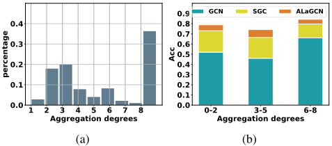
We first open up our model to see the distribution of nodewise aggregation degree in Figure 4 when the max aggregation degree is set to 9. We only consider nodes with a relatively large z value as actively performing aggregation in the target layer. From Figure 4a, we see that around 13 of the nodes choose to have an aggregation degree of 9 with another mode appearing near L = 3. We then divide all nodes into 3 groups based on their associated aggregation degree. Figure
| Methods | Cora | CiteSeer | PubMed |
|---|---|---|---|
| DeepWalk | 67.2 | 43.2 | 65.3 |
| Planetoid | 75.7 | 64.7 | 77.2 |
| LP | 68.0 | 45.3 | 63.0 |
| CS-GNN | 70.1 (2) | 56.0 (2) | 73.6 (2) |
| GResNet | 81.7 (5) | 67.3 (4) | 78.5 (7) |
| Co/self-train | 79.8 (2) | 69.9 (2) | 77.0 (2) |
| PairNorm | 81.2 (5) | 66.5 (3) | 79.8 (9) |
| APPNP | 84.3 (2) | 68.8 (2) | 78.7 (2) |
| GCN | 81.6 (2) | 69.2 (2) | 77.8 (2) |
| GraphSage | 81.3 (2) | 69.7 (2) | 77.2 (2) |
| SGC | 81.8 (3) | 68.9 (2) | 77.5 (3) |
| ALaGCN | 82.9 (3) | 70.9 (3) | 79.6 (6) |
| GAT | 83.8 (2) | 71.1 (2) | 77.6 (2) |
| ALaGAT | 85.0 (2) | 71.5 (2) | 78.1 (7) |
4b shows that ALaGCN outperforms both GCN and SGC in all three groups with a larger gap in the first two groups.
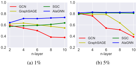
Figure 5 shows how the predicted accuracy changes with max aggregation degree L. The performance of GCN and GraphSAGE decreases significantly with the number of layers as a results of overfitting and over-smoothing. SGC's performance does not significantly degrade but allowing nodes to differ in aggregation degree still improves performance.
5.4 Efficiency
For our proposed metrics, computing the neighborhood entropy for all nodes has the complexity of O(|N|dC) where |N| is the total number of nodes, d is the average degree of the graph and C is the total number of classes for prediction. Center-neighbor similarity has a complexity of O(|N|d). Both computation complexities are on par with the neighborhood aggregation operation in GCN, which is O(|N|d). During inference, we may fix the thresholds and turn off aggregation whenever z is low. This leads to a tradeoff between the time required to check the metrics and the time used for performing aggregation. On graphs with clear community structure, this may result in faster inference.
| Dataset | GCN | GAT | ALaGCN |
|---|---|---|---|
| Cora | 1x (24.4 ms) | 5.95x | 1.38x |
| CiteSeer | 1x (23.1ms) | 5.30x | 1.45x |
| PubMed | 1x (60.8ms) | 21.3x | 1.49x |
As shown in Table 5, our ALaGCN model scales similarly to GCN with an overhead of checking the metrics. Sophisticated models like GAT, on the other hand, have significantly longer run times, especially on larger datasets.
6 RelatedWork
Previous work [Li et al., 2018] showed that doing too much aggregation on the entire graph will reduce all node features to a fixed point, and coined this phenomenon as 'oversmoothing'. It was followed by [Chen et al., 2020] and [Zhao and Akoglu, 2020], which give quantitative measurements of over-smoothing, and [Hou et al., 2020], which measures how much information is leveraged from neighborhood aggregation. Our work, on the other hand, is based on the intuition that the effect of neighborhood aggregation can vary across individual nodes. Focusing on a local perspective, we analyze and address the circumstances when neighborhood aggregation is harmful or unnecessary for each individual node.
Some GNN models have attempted to improve neighborhood aggregation by enlarging the scope of the neighborhood [Li et al., 2018; Klicpera et al., 2019]. Another line of work tries to balance the usage of neighborhood information and original node features [Hou et al., 2020; Chen et al., 2020]. In contrast, our model makes a more principled yet adaptive adjustment to balance graph links and features, by allowing a node to access a large scope of neighbors only when aggregation is expected to be helpful.
7 Conclusion and FutureWork
In this paper, we analyze a key component prevalent in GNN models: the neighborhood aggregation operation. We observe that in a network, different nodes may require different aggregation degrees to reach a correct prediction. Excessive aggregation may be redundant or even harmful, leading to the over-smoothing phenomenon, where all nodes eventually converge to the same fixed point. To characterize when neighborhood aggregation may be unnecessary, we propose two metrics: neighborhood entropy and center-neighbor similarity. We show empirically and theoretically that the proposed metrics can successfully identify nodes that do not benefit from neighborhood aggregation. Furthermore, we design a model ALaGCN and its attention-enhanced sibling ALaGAT that tests for the proposed metrics at each layer before performing aggregation. Our experiments show that by adding this test, we can achieve consistent improvement over GCN and the best or near-best performance among a range of GNN-based models.
One potential direction for future work is to extend the analysis to other tasks, such as graph classification and link prediction.
Acknowledgements
We thank Xumeng Chen for helping with the experiments. Research was sponsored in part by US DARPA KAIROS Program No. FA8750-19-2-1004 and SocialSim Program No. W911NF-17-C-0099, National Science Foundation IIS 16-18481, IIS 17-04532, and IIS-17-41317, and DTRA HDTRA11810026.
@inproceedings{ijcai2020p181,
  title     = {When Do GNNs Work: Understanding and Improving Neighborhood Aggregation},
  author    = {Xie, Yiqing and Li, Sha and Yang, Carl and Wong, Raymond Chi-Wing and Han, Jiawei},
  booktitle = {Proceedings of the Twenty-Ninth International Joint Conference on
               Artificial Intelligence, {IJCAI-20}},
  publisher = {International Joint Conferences on Artificial Intelligence Organization},
  editor    = {Christian Bessiere},
  pages     = {1303--1309},
  year      = {2020},
  month     = {7},
  note      = {Main track},
  doi       = {10.24963/ijcai.2020/181},
  url       = {https://doi.org/10.24963/ijcai.2020/181},
}
TY - CPAPER TI - When Do GNNs Work: Understanding and Improving Neighborhood Aggregation AU - Xie, Yiqing AU - Li, Sha AU - Yang, Carl AU - Wong, Raymond Chi-Wing AU - Han, Jiawei T2 - Proceedings of the Twenty-Ninth International Joint Conference on Artificial Intelligence, IJCAI-20 PB - International Joint Conferences on Artificial Intelligence Organization PY - 2020 SP - 1303 EP - 1309 DO - 10.24963/ijcai.2020/181 UR - https://doi.org/10.24963/ijcai.2020/181 ER -Copied
Machine-readable versions of this paper, for tools and AI agents:





