
An End-to-End Optimal Trade Execution Framework based on Proximal Policy Optimization
Proceedings of the Twenty-Ninth International Joint Conference on Artificial Intelligence. Special Track on AI in FinTech. Pages 4548-4554.
https://doi.org/10.24963/ijcai.2020/627
Keywords
- AI for trading: AI for algorithmic trading
- Foundation for AI in FinTech: Reinforcement learning for FinTech
Abstract
In this article, we propose an end-to-end adaptive framework for optimal trade execution based on Proximal Policy Optimization (PPO). We use two methods to account for the time dependencies in the market data based on two different neural network architecture: 1) Long short-term memory (LSTM) networks, 2) Fully-connected networks (FCN) by stacking the most recent limit orderbook (LOB) information as model inputs. The proposed framework can make trade execution decisions based on level-2 limit order book (LOB) information such as bid/ask prices and volumes directly without manually designed attributes as in previous research. Furthermore, we use a sparse reward function, which gives the agent reward signals at the end of each episode as an indicator of its relative performances against the baseline model, rather than implementation shortfall (IS) or a shaped reward function. The experimental results have demonstrated advantages over IS and the shaped reward function in terms of performance and simplicity. The proposed framework has outperformed the industry commonly used baseline models such as TWAP, VWAP, and AC as well as several Deep Reinforcement Learning (DRL) models on most of the 14 US equities in our experiments.
- Standard Deviation Model Name BA CRM FB GOOG GS MCD MSCI NVDA PEP PYPL QCOM TSLA TWLO WMT TWAP 335.05 885.62 4,154.47 707.03 92.74 221.72 159.14 478.18 1,058.16 681.91 2,913.72 203.00 196.88 1,442.92 VWAP 503.64 1,366.18 14,936.29 1,394.18 190.89 420.70 220.25 726.23 2,389.84 2,587.93 27,131.03 462.24 341.32 6,699.03 AC 335.80 894.99 4,517.32 707.40 93.19 222.10 159.59 479.65 1,058.48 776.66 4,724.56 210.49 215.42 1,456.07 DQN (Ning2018) 506.22 1,086.15 5,298.78 962.25 64.98 183.17 641.79 629.95 5,082.65 1,242.17 6,890.66 239.12 204.75 1,758.85 DQN (Lin2019) 326.62 830.79 4,117.55 696.35 91.07 214.50 642.64 454.73 1,033.27 631.29 2,821.33 226.80 196.34 1,386.26 DQN Sparse (Lin2019) 343.27 842.26 4,245.49 719.14 96.03 223.89 161.44 503.98 1,071.55 753.93 3,091.98 226.49 196.58 1,479.68 PPO Dense 345.79 836.57 4,379.35 708.64 92.68 221.73 159.47 478.18 1,153.07 672.30 3,795.95 244.20 204.27 1,599.52 PPO Stack 322.24 812.22 3,929.08 630.45 93.08 344.90 149.68 573.88 1,013.80 610.21 2,551.04 200.54 206.20 1,405.03 PPO LSTM 294.09 859.73 4,462.66 690.63 113.71 576.29 145.73 431.11 997.11 624.24 2,654.01 183.42 186.11 1,355.22
- [Almgren and Chriss, 2000] Robert Almgren and Neil Chriss. Optimal execution of portfolio transactions. Journal of Risk, 3:5-40, 2000.
- [Berkowitz et al., 1988] Stephen A. Berkowitz, Dennis E. Logue, and Eugene A. Noser Jr. The total cost of transac- tions on the nyse. Journal of Finance, 43(1):97-112, March 1988.
- [Bertsimas and Lo, 1998] Dimitris Bertsimas and Andrew W. Lo. Optimal control of execution costs. Journal of Finan- cial Markets, 1(1):1-50, April 1998.
- [Hendricks and Wilcox, 2014] Dieter Hendricks and Diane Wilcox. A reinforcement learning extension to the almgren- chriss framework for optimal trade execution. In Proceed- ings from IEEE Conference on Computational Intelligence for Financial Economics and Engineering, pages 57-464, London, UK, March 2014. IEEE.
- [Hochreiter and Schmidhuber, 1997] Sepp Hochreiter and Jürgen Schmidhuber. Long short-term memory. Neural computation, 9(8):1735-1780, 1997.
- [Huberman and Stanzl, 2005] Gur Huberman and Werner Stanzl. Optimal liquidity trading. Review of Finance, 9(2):165-200, 2005.
- [Kakade et al., 2004] Sham M. Kakade, Michael Kearns, Yishay Mansour, and Luis E. Ortiz. Competitive algo- rithms for vwap and limit order trading. In Proceedings of the ACM Conference on Electronic Commerce, New York, NY, 2004.
- [Liaw et al., 2018] Richard Liaw, Eric Liang, Robert Nishi- hara, Philipp Moritz, Joseph E Gonzalez, and Ion Stoica. Tune: A research platform for distributed model selection and training. arXiv preprint arXiv:1807.05118, 2018.
- [Lin and Beling, 2019] Siyu Lin and Peter A. Beling. Op- timal liquidation with deep reinforcement learning. In 33rd Conference on Neural Information Processing Systems (NeurIPS 2019) Deep Reinforcement Learning Workshop, Vancouver, Canada, 2019.
- [Mnih et al., 2013] Volodymyr Mnih, Koray Kavukcuoglu, David Silver, Alex Graves, Ioannis Antonoglou, Daan Wier- stra, and Martin Riedmiller. Playing atari with deep rein- forcement learning. arXiv preprint arXiv:1312.5602, 2013.
- [Mnih et al., 2015] Volodymyr Mnih, Koray Kavukcuoglu, David Silver, Andrei A. Rusu, Joel Veness, Marc G. Belle- mare, Alex Graves, Martin Riedmiller, Andreas K. Fid- jeland, Georg Ostrovski, Stig Petersen, Charles Beattie, Amir Sadik, Ioannis Antonoglou, Helen King, Dharshan Kumaran, Daan Wierstra, Shane Legg, and Demis Hassabis. Human-level control through deep reinforcement learning. Nature, 518:529-533, February 2015.
- [Nevmyvaka et al., 2006] Yuriy Nevmyvaka, Yi Feng, and Michael Kearns. Reinforcement learning for optimal trade execution. In Proceedings of the 23rd International Confer- ence on Machine Learning, pages 673-68, Pittsburgh, PA, June 2006. Association for Computing Machinery. Ning et al., 2018]
- Brian Ning, Franco Ho Ting Ling, and Sebastian Jaimungal. Double deep q-learning for optimal execution. arXiv:1812.06600, 2018.
- [Schulman et al., 2017] John Schulman, Filip Wolski, Pra- fulla Dhariwal, Alec Radford, and Oleg Klimov. Proximal policy optimization algorithms. arXiv:1811.08540v2, 2017.
References were extracted automatically from the PDF and may contain errors.
Full text extracted automatically from the PDF; figures, tables and equations may differ. The PDF is the version of record.
1 Introduction
In the modern financial market, electronic trading has gradually replaced the traditional floor trading and is constituting a majority of the overall trading volumes. Nowadays, brokerage firms compete intensively with each other to provide better execution quality to retail or institutional investors. Optimal trade execution, which concerns how to minimize trade execution costs of trading a certain amount of shares within a specified period, is a critical factor of execution quality.
From the regulatory perspective, brokers are legally required to execute orders on behalf of their clients to ensure the best execution possible. In the US, such practices are monitored by the Securities and Exchange Commission (SEC) and Financial Industry Regulatory Authority (FINRA). In Europe, MiFID II, a legislative framework instituted by the European Union, regulates financial markets and improves protections for investors.
1.1 RelatedWork
Bertsimas and Lo are the pioneers in the realm of optimal trade execution. They use a dynamic programming approach to find an explicit closed-form solution by minimizing trade execution costs of large transactions over a fixed trading period [Bertsimas and Lo, 1998]. Huberman, Stanzl [Huberman and Stanzl, 2005] and Almgren, Chriss [Almgren and Chriss, 2000] extend their work by introducing transaction costs, more complex price impact functions, risk aversion parameters. The closedform analytical solutions, however, have strong assumptions on the underlying price movement or distributions. In addition to the closed-form solutions, the time-weighted average price (TWAP) strategy and volume-weighted average price (VWAP) strategy are prevalent among practitioners in financial markets [Berkowitz et al., 1988]. The TWAP and VWAP strategies have few assumptions; however, both strategies are not able to learn from historical data.
Reinforcement learning (RL) seems to be a natural choice for the optimal trade execution problem, as it enables the trading agent to interact with the market and to learn from its experiences and has fewer assumptions on the price dynamics than the closed-form solutions. Nevmyvaka, Feng, and Kearns have published the first large-scale empirical application of RL to optimal trade execution problems [Nevmyvaka et al., 2006]. Hendricks and Wilcox propose to combine the Almgren and Chriss model (AC) and RL algorithm and to create a hybrid framework mapping the states to the proportion of the ACsuggested trading volumes [Hendricks and Wilcox, 2014].
To address the high dimensions and the complexity of the underlying dynamics of the financial market, Ning et al. [Ning et al., 2018] adapt and modify the Deep Q-Network (DQN) [Mnih et al., 2015] for optimal trade execution, which combines the deep neural network and the Q-learning, and can address the curse of dimensionality challenge faced by Q-learning. Lin and Beling [Lin and Beling, 2019] analyze and demonstrate the flaws when applying a generic Q-learning algorithm and propose a modified DQN algorithm to address the zero-ending inventory constraint.
However, the researchers in previous research all use manually designed attributes which adds a further burden to the system development in the real-world, since feature engineering requires significant domain knowledge and efforts. We desire an end-to-end optimal trade execution system without feature engineering.
Previously, most researchers use Implementation Shortfall (IS) as the immediate reward signal. Lin and Beling [Lin and Beling, 2019] point out the disadvantages of IS as a reward signal and propose a shaped reward structure. Even though they claim that the proposed reward function generalizes reasonably well on the stocks, we prefer a much simpler reward structure, which requires minimal domain knowledge and efforts on designing its structure and tuning its parameters with less risk of overfitting.
1.2 Our Contribution
Our main contributions are: 1) We propose an end-to-end optimal trade execution framework which can account for temporal correlations and make decisions based on raw level2 market microstructure data 1 instead of manually designed attributes. 2) We propose a sparse reward signal and demonstrate its advantage over IS and the shaped reward structure proposed in previous research. 3) We perform an extensive experiment to demonstrate the advantages of our framework over several DRL agorithms including Ning et al's [2018] and Lin and Beling's [2019] algorithms and their variants as well as three commonly used algorithms in the financial industry: TWAP, VWAP, and AC model.
2 A PPO Formulation to Optimal Trade Execution
The PPO algorithm is a policy gradient algorithm proposed by OpenAI [Schulman et al., 2017], and it becomes one of the most popular RL methods due to its state-of-the-art performance as well as its sample efficiency and easy implementation. To optimize policies, it alternates between sampling data and optimizing a "surrogate" objective function.
2.1 Preliminaries
PPO is an on-policy algorithm and applies to both discrete and continuous action spaces. PPO-clip updates policies via
where π is the policy, θ is the policy parameter, k is the kth step, a and s are action and state respectively. It typically takes multiple steps of SGD to optimize the objective L
where Aπθk (s, a) is the advantage estimator. The clip term in Equation 2 clips the probability ratio and prevents the new policy going far away from the old policy 2 [Schulman et al., 2017].
1 top 5 levels bid/ask prices and volumes
2 https://spinningup.openai.com/en/latest/algorithms/ppo.html
| Ticker | Trading Shares | Ticker | Trading Shares |
|---|---|---|---|
| FB | 6000 | GS | 300 |
| GOOG | 300 | CRM | 1200 |
| NVDA | 600 | BA | 300 |
| MSCI | 300 | MCD | 600 |
| TSLA | 300 | PEP | 1800 |
| PYPL | 2400 | TWLO | 600 |
| QCOM | 7200 | WMT | 3600 |
2.2 ProblemFormulation
In this section, we provide the PPO formulation for the optimal trade execution problem and describe the state, action, reward, and the algorithm used in the experiment.
States
Previously, researchers use manually designed attributes to represent the financial market state, which can be inefficient and time-consuming in real-world applications. In this article, we propose to use 1) Public state: market microstructure variables including top 5 bid/ask prices and associated volumes; 2) Private state: remaining inventory and elapsed time.
Actions
In this article, we choose different numbers of shares to trade based on the liquidity of the stock market. As the purpose of the research is to evaluate the capability of the proposed framework to balance the liquidity risk and timing risk, we choose the total number of shares to ensure that the TWAP orders 3 are able to consume at least the 2nd best bid price on average. The total shares to trade for each stock are illustrated in Table 1. In the optimal trade execution framework, we set the range of actions from 0 to 2TWAP and set the minimal trading volume for each stock, respectively.
Rewards
In previous work [Nevmyvaka et al., 2006][Hendricks and Wilcox, 2014][Ning et al., 2018], researchers use the IS 4 , a commonly used metric to measure execution gain/loss, as the immediate reward received after execution at each nonterminal step. There is a common misconception that the IS is a direct optimization goal. The IS compares the model performance to an idealized policy that assumes infinite liquidity at the arrival price. In the real world, brokers often use TWAP and VWAP as benchmarks. IS is usually used as the optimization goal because TWAP and VWAP prices could only be computed until the end of the trading horizon and cannot be used for real-time optimization. Essentially, IS is just a surrogate reward function, but not a direct optimization goal. Hence, a reward structure is good as long as it can improve model performance.
Lin and Beling [Lin and Beling, 2019] point out that IS reward is noisy and nonstationary, which makes the learning process difficult. They propose a shaped reward structure and fine-tune it on Facebook training data. Although their proposed reward structure seems to generalize reasonably well on the rest equities as demonstrated in their article, the designing of a complicated reward structure is time-consuming and has a risk of overfitting in real-world applications.
3 TWAP order = Total number of shares to trade Total # of periods
4 Implementation Shortfall=arrival price×traded volume - executed price×traded volume.
In contrast to previous approaches, we use a sparse reward, which only gives the agent a reward signal based on its relative performance compared against the TWAP baseline model.
f (x) = ⎧⎪⎪⎨⎪⎪⎩ -1, if t = T -1 and ISPPO(T) < ISTWAP(T) 0, if t = T - 1 and ISTWAP(T) <= ISPPO(T) < 1.1 ∗ ISTWAP(T) 1, if t = T - 1 and ISPPO(T) >= 1.1 ∗ ISTWAP(T) 0, if 1 <= t < T - 1Zero Ending Inventory Constraint
In the real world business, the brokers receive contracts or directives from their clients to execute a certain amount of shares within a specific time. For the brokers, it is mandatory to liquidate all the shares by the end of the trading period. Lin and Beling [Lin and Beling, 2019] modify the Q-function update to combine the last two steps for Q-function estimation to incorporate the zero-ending inventory constraint. We leverage their methods by combining the last two steps.
Assumptions
The most important assumption in our experiment is that the actions that DRL agent takes have only a temporary market impact, and the market is resilient and will bounce back to the equilibrium level at the next time step. This assumption also suggests that the DRL agent's actions do not affect the behaviors of other market participants. The market resilience assumption is the core assumption of this article and also all previous research applying RL for optimal trade execution problems [2006][2014][2018]. The reason is that we are training and testing on the historical data and cannot account for the permanent market impact. However, the equities we choose in the article are liquid, and the actions are relatively small compared with the market volumes. Therefore, the assumption should be reasonable.
Secondly, we ignore the commissions and exchange fees as our research is primarily aimed at institutional investors, and those fees are relatively small fractions and are negligible. The ignorance of such fees is also the practice of previous research [2006][2014][2018]. Thirdly, we apply a quadratic penalty if the trading volume exceeds the available volumes of the top 5 bids. Fourthly, the remaining unexecuted volumes will be liquidated all at once at the last time step to ensure the execution of all the shares. Fifthly, we also assume direct and fast access to exchanges with no order arrival delays. Finally, if multiple actions result in the same reward, we choose the maximum action (trading volumes). The rationale is that we would like to trade as quickly as possible while not encountering too much loss.
Most of the assumptions are also the core assumptions in previous research [2006][2014][2018] because we need a highfidelity market simulation environments or data collected by implementing the DRL algorithm in the real market rather than historical data to account for these factors such as order delays, permanent market impact, and agent interactions, etc..
2.3 PPOArchitecture
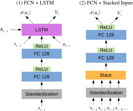
Unlike the DQN algorithm, the PPO algorithm optimizes over the policy πt directly and finds the optimal state-value function V∗ t . We leverage Ray's Tune platform to select the network architecture and hyperparameters by comparing model performances on Facebook data only, which is equivalent to ablation studies. The selected network architectures are illustrated in Figure 1.
Network Architecture
In the PPO algorithm, we have implemented two network architectures: 1) FCN with two hidden layers, 128 hidden nodes in each hidden layer, and ReLU activation function in each hidden node. The input layer has 22 nodes, including private attributes such as remaining inventory and time elapsed as well as the LOB attributes such as 5-level bid/ask prices and volumes. After that, we concatenate the model output and the previous reward and action and feed them to a LSTM network with cell size of 128. The LSTM outputs the policy πt and the state-value function V∗ t . 2) FCN with the same settings as 1), except that we stack the most recent LOB attributes as model inputs. We choose the Adam optimizer for weights optimization.
Long Short-Term Memory
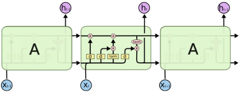
Unlike the feedforward neural networks, LSTM has feedback connections, which allows it to store information and identify temporal patterns. LSTM networks are composed of a number of cells, and an input gate, an output gate, and a forget gate within each cell regulate the flow of information into and out of the cell, as demonstrated in Figure 2. It was proposed by Sepp Hochreiter and J¨urgen Schmidhuber to solve the exploding and vanishing gradient problems encountered by the traditional recurrent neural network (RNN) [1997]. Instead of manually designing attributes to represent the temporal patterns, we leverage LSTM to process the sequential LOB data and automatically identify temporal patterns within the data.
2.4 Experimental Methodology and Settings
In our experiments, we apply the proposed PPO algorithms on 14 stocks including Facebook (FB), Google (GOOG), Nvidia (NVDA), Msci (MSCI), Tesla (TSLA), PayPal (PYPL), Qualcomm (QCOM), Goldman Sachs (GS), Salesforce.com (CRM), Boeing (BA), Mcdonald's Corp (MCD), PepsiCo (PEP), Twilio (TWLO), and Walmart (WMT) which cover technology, financial and retail industries. We tune the hyperparameters on FB only and apply the same neural network architecture to the remaining stocks due to limited computing resources. The experiment follows the steps below.
- We obtain one-year millisecond Trade and Quote (TAQ) data of 14 stocks above fromWRDS and reconstruct it into the LOB. Then, we split the data into training (January-September) and test sets (October-December). We set the execution horizon to be 1 minute, and the minimum trading interval to be 5 seconds.
- The hyperparameters 5 are tuned on FB only due to the limited computing resources. After fine-tuning, we apply the PPO architecture and hyperparameters to the rest stocks.
- Upon the completion of training, we check the average episode rewards' progression. Then, we apply the learned policies to the testing data and compare the average episode rewards and the distribution of rewards against TWAP, VWAP, and AC models as well as several DRL algorithms.
Algorithm Implementation
In our experiment, we implement a distributed version of the PPO algorithm in Ray RLlib and fine-tune the hyperparameters such as the neural network architecture, learning rate, etc. using Tune, a research platform developed by Liaw et al. [2018]. 6
3 Experimental Results
In this section, we present the proposed framework's performance and compare it with the TWAP, VWAP, AC model as well as several DRL models. Our proposed framework converges fast and has significantly outperformed the baseline models on most stocks during the backtesting. In our experiment, we apply DeepMind's framework to assess the stability in the training phase and the performance evaluation in the backtesting [Mnih et al., 2013].
3.1 Data Sources
We use the NYSE daily millisecond TAQ data from January 1st, 2018 to December 31st, 2018, downloaded fromWRDS. The TAQ data is used to reconstruct the LOB. Only the top 5 price levels from both seller and buyer sides are kept and aggregated at 5 seconds, which is the minimum trading interval.
5 Please refer to the appendix for the chosen hyperparameters
6 https://ray.readthedocs.io/en/latest/rllib.html
3.2 Algorithms
TWAP: The shares are equally divided across time.
VWAP: The shares are traded at a price which closely tracks the VWAP [2004].
AC: AC is defined in [2000]. For a fair comparison with AC, we set its permanent price impact parameter to 0.
DDQN (Ning2018): This is a variant of [2018] with 51 states defined in [2019]. The neural network architecture is also different and has been tuned for optimal performances. It uses the same reward function and training process as [2018].
DQN (Lin2019): The modified DQN algorithm proposed by [Lin and Beling, 2019].
DQN Sparse (Lin2019): A variant of DQN (Lin2019) which uses the sparse reward function defined in Section 2.2.
PPO Dense: The PPO algorithm uses the 51 states and shaped rewards defined in [2019].
PPO Stack: The PPO algorithm stacks the most recent LOB states as model inputs.
PPO LSTM: The PPO algorithm uses LSTM to extract temporal patterns within market data.
3.3 Training and Stability
Assessing the stability and the model performance in the training phase is straightforward in supervised learning by evaluating the training and testing samples. However, it is challenging to evaluate and track the RL agent's progress during training, since we usually use the average episode rewards gained by the agent over multiple episodes as the evaluation metric to track the agent's learning progress. The average episode reward is usually noisy since the updates on the parameters of the policy can seriously change the distribution of states that the DRL agent visits.
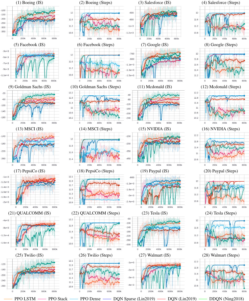
In Figure 3, we observe that the DRL agents converge fast in less than 200,000 steps 7 . The PPO+LSTM and the PPO+Stack converge to higher average IS values on most stocks, while having shorter trading lengths. It indicates that not only do they reduce the execution costs, but also they trade more quickly to avoid timing risks. Ning et al's method has demonstrated great oscillations on some stocks which could be dangerous in real world applications.
3.4 Main Evaluation and Backtesting
To evaluate the performance of the trained PPO algorithms, we apply them to the test samples from October 2018 to December 2018 for all the 14 stocks and compare their performances with TWAP, VWAP, and AC model as well as several DRL models. We report the mean of ∆IS = ISModel - ISTWAP (in US dollars), standard deviation of ISModel, and gain-loss ratio (GLR)
The statistical results for all the stocks are summarized in Table 2. We observe that the proposed PPO LSTM/Stack algorithms outperform the other models most of time, while maintaining relative smaller standard deviations. In the experiments, we also find out that DQN does not work well with the sparse rewards (see DQN (Lin2019) vs DQN Sparse (Lin2019)). We highlight the top 2 performers in bold font. Also, we highlight the extreme divergence in red. Although Ning et al.'s method has good performances on a few stocks, it has demonstrated great oscillations and even divergence on some stocks. Such oscillations and instabilities could be dangerous in real-world applications, and should be avoided.
7 Odd index represents the learning curves for the IS, while even index represents for the learning curves for the total # of steps to complete the trades
| Model Name | Mean | |||||||||||||
|---|---|---|---|---|---|---|---|---|---|---|---|---|---|---|
| BA | CRM | FB | GOOG | GS | MCD | MSCI | NVDA | PEP | PYPL | QCOM | TSLA | TWLO | WMT | |
| TWAP | 0.00 | 0.00 | 0.00 | 0.00 | 0.00 | 0.00 | 0.00 | 0.00 | 0.00 | 0.00 | 0.00 | 0.00 | 0.00 | 0.00 |
| VWAP | 49.66 | -141.42 | -4,040.78 | -65.41 | -12.58 | -7.89 | 34.94 | -31.46 | -77.54 | -459.28 | -6,737.10 | -65.04 | -41.27 | -1,376.78 |
| AC | -0.78 | -3.34 | -40.26 | -0.92 | -0.16 | -0.13 | -0.34 | -1.32 | -0.34 | -8.88 | -127.87 | -1.21 | -2.96 | -2.24 |
| DQN (Ning2018) | 91.35 | 16.65 | -545.49 | 183.63 | 42.41 | 104.18 | -770.09 | 70.33 | -15,074.82 | -30.81 | -1,056.94 | 46.03 | 49.77 | 140.32 |
| DQN (Lin2019) | 16.21 | 9.05 | 54.08 | 28.43 | 2.40 | 11.86 | -770.24 | 19.50 | 38.45 | 47.35 | 152.02 | 3.30 | 4.63 | 99.56 |
| DQN Sparse (Lin2019) | -6.82 | -4.09 | -110.18 | -13.79 | -1.58 | 2.17 | -2.83 | -3.31 | -21.55 | -73.89 | -78.97 | 1.04 | -0.83 | -43.13 |
| PPO Dense | -3.35 | -0.19 | -33.32 | -0.75 | -0.02 | 0.00 | -0.18 | 0.00 | -132.48 | -0.26 | -52.88 | -11.12 | -28.31 | -171.49 |
| PPO Stack | 13.35 | 22.06 | 451.80 | 147.44 | 13.49 | -46.56 | 36.09 | -60.70 | 122.09 | 66.11 | 412.20 | 30.12 | 16.08 | 224.23 |
| PPO LSTM | 72.53 | 101.87 | 128.23 | 18.06 | -1.81 | -178.71 | 35.50 | 71.32 | 76.78 | 114.38 | 321.43 | 46.96 | 21.94 | 153.58 |
| Standard Deviation | ||||||||||||||
| Model Name | BA | CRM | FB | GOOG | GS | MCD | MSCI | NVDA | PEP | PYPL | QCOM | TSLA | TWLO | WMT |
| TWAP | 335.05 | 885.62 | 4,154.47 | 707.03 | 92.74 | 221.72 | 159.14 | 478.18 | 1,058.16 | 681.91 | 2,913.72 | 203.00 | 196.88 | 1,442.92 |
| VWAP | 503.64 | 1,366.18 | 14,936.29 | 1,394.18 | 190.89 | 420.70 | 220.25 | 726.23 | 2,389.84 | 2,587.93 | 27,131.03 | 462.24 | 341.32 | 6,699.03 |
| AC | 335.80 | 894.99 | 4,517.32 | 707.40 | 93.19 | 222.10 | 159.59 | 479.65 | 1,058.48 | 776.66 | 4,724.56 | 210.49 | 215.42 | 1,456.07 |
| DQN (Ning2018) | 506.22 | 1,086.15 | 5,298.78 | 962.25 | 64.98 | 183.17 | 641.79 | 629.95 | 5,082.65 | 1,242.17 | 6,890.66 | 239.12 | 204.75 | 1,758.85 |
| DQN (Lin2019) | 326.62 | 830.79 | 4,117.55 | 696.35 | 91.07 | 214.50 | 642.64 | 454.73 | 1,033.27 | 631.29 | 2,821.33 | 226.80 | 196.34 | 1,386.26 |
| DQN Sparse (Lin2019) | 343.27 | 842.26 | 4,245.49 | 719.14 | 96.03 | 223.89 | 161.44 | 503.98 | 1,071.55 | 753.93 | 3,091.98 | 226.49 | 196.58 | 1,479.68 |
| PPO Dense | 345.79 | 836.57 | 4,379.35 | 708.64 | 92.68 | 221.73 | 159.47 | 478.18 | 1,153.07 | 672.30 | 3,795.95 | 244.20 | 204.27 | 1,599.52 |
| PPO Stack | 322.24 | 812.22 | 3,929.08 | 630.45 | 93.08 | 344.90 | 149.68 | 573.88 | 1,013.80 | 610.21 | 2,551.04 | 200.54 | 206.20 | 1,405.03 |
| PPO LSTM | 294.09 | 859.73 | 4,462.66 | 690.63 | 113.71 | 576.29 | 145.73 | 431.11 | 997.11 | 624.24 | 2,654.01 | 183.42 | 186.11 | 1,355.22 |
| Model | GLR | |||||||||||||
| Name | BA | CRM | FB | GOOG | GS | MCD | MSCI | NVDA | PEP | PYPL | QCOM | TSLA | TWLO | WMT |
| TWAP | - | - | - | - | - | - | - | - | - | - | - | - | - | - |
| VWAP | 0.59 | 0.46 | 0.16 | 0.46 | 0.46 | 0.49 | 0.72 | 0.51 | 0.40 | 0.22 | 0.08 | 0.40 | 0.41 | 0.17 |
| AC | 0.04 | 0.02 | 0.00 | 0.10 | 0.16 | 0.11 | 0.15 | 0.06 | 0.18 | 0.00 | 0.01 | 0.10 | 0.05 | 0.02 |
| DQN (Ning2018) | 0.69 | 0.66 | 0.57 | 0.78 | 2.96 | 2.27 | 0.08 | 0.73 | 0.01 | 0.44 | 0.33 | 1.40 | 1.16 | 1.14 |
| DQN (Lin2019) | 1.47 | 1.18 | 1.04 | 1.28 | 1.40 | 2.00 | 0.09 | 1.54 | 1.49 | 2.13 | 1.53 | 1.27 | 1.11 | 1.94 |
| DQN Sparse (Lin2019) | 0.46 | 1.00 | 0.96 | 0.44 | 0.99 | 1.01 | 0.55 | 0.98 | 0.49 | 0.36 | 0.98 | 1.01 | 1.03 | 0.30 |
| PPO Dense | 0.21 | 0.26 | 0.41 | 0.26 | 0.96 | 0.52 | 0.34 | - | 1.01 | 0.45 | 0.65 | 0.88 | 0.47 | 0.87 |
| PPO Stack | 1.11 | 1.46 | 2.07 | 1.63 | 0.93 | 0.39 | 1.39 | 0.67 | 1.35 | 1.49 | 2.38 | 1.69 | 0.84 | 1.22 |
| PPO LSTM | 1.54 | 1.43 | 0.63 | 1.34 | 0.58 | 0.23 | 1.55 | 1.21 | 1.30 | 1.64 | 1.63 | 1.35 | 1.49 | 1.32 |
We exclude the methods proposed by [Nevmyvaka et al., 2006] and [Hendricks and Wilcox, 2014] from the performance comparison for several reasons: 1) Traditional Reinforcement Learning is not scalable to high dimensional problems. 2) Both articles are using market data quite a while ago 8 . It's difficult to evaluate the effectiveness of their methods, since the dynamics of market microstructure have already changed dramatically in the past few years.
4 Conclusion and FutureWork
In this article, we propose an end-to-end optimal trade execution framework based on PPO. In our experiments, we have demonstrated that the proposed framework is able to outperform TWAP, VWAP, AC model as well as other DRL models using raw level-2 market data. Additionally, we have also demonstrated that DRL agents are able to learn good execution strategies even with the sparse rewards. The experimental results are significant and indicate the possibility of learning optimal trade execution policies from the raw market microstructure data without feature engineering.
8 Nevmyvaka et al.'s method was tested on three NASDAQ stocks, AMZN, NVDA, and QCOM, before 2006. Hendricks and Wilcox's method was tested on three South Africa's stocks, SBK, AGL, and SAB, in 2012
In the future, we are planning to relax the assumption that the DRL agent's actions are independent of other market participants' actions and model the interactions of multiple DRL agents and their collective decisions in the market.
A Hyperparameters
We fine-tuned the hyperparameters on FB only, and we did not perform an exhaustive grid search on the hyperparameter space, but rather to draw random samples from the hyperparameter space due to limited computing resources. Finally, we choose the hyparameters listed in Table 3.
| Hyperparameter | PPO LSTM | PPO Stack |
|---|---|---|
| Minibatch size | 32 | 32 |
| Sample batch size | 5 | 5 |
| Train batch size | 240 | 240 |
| Discount factor | 1 | 1 |
| Learning rate | linearly annealing between 5e-5 and 1e-5 | linearly annealing between 5e-5 and 1e-5 |
| KL coeff | 0.2 | 0.2 |
| VF loss coeff | 1 | 1 |
| Entropy coeff | 0.01 | 0.01 |
| Clip param | 0.2 | 0.2 |
| Hidden layers | 2 hidden layers with 128 hidden nodes each | 2 hidden layers with 128 hidden nodes each |
| Activation functions | Relu for hidden layers and linear for output layer | Relu for hidden layers and linear for output layer |
| # input/output nodes | Input: 22; output: 51 | Input: 82; output: 51 |
| Maximum sequence length | 12 | None |
| LSTM cell size | 128 | None |
| Stack steps | None | 4 |
@inproceedings{ijcai2020p627,
  title     = {An End-to-End Optimal Trade Execution Framework based on Proximal Policy Optimization},
  author    = {Lin, Siyu and Beling, Peter A.},
  booktitle = {Proceedings of the Twenty-Ninth International Joint Conference on
               Artificial Intelligence, {IJCAI-20}},
  publisher = {International Joint Conferences on Artificial Intelligence Organization},
  editor    = {Christian Bessiere},
  pages     = {4548--4554},
  year      = {2020},
  month     = {7},
  note      = {Special Track on AI in FinTech},
  doi       = {10.24963/ijcai.2020/627},
  url       = {https://doi.org/10.24963/ijcai.2020/627},
}
TY - CPAPER TI - An End-to-End Optimal Trade Execution Framework based on Proximal Policy Optimization AU - Lin, Siyu AU - Beling, Peter A. T2 - Proceedings of the Twenty-Ninth International Joint Conference on Artificial Intelligence, IJCAI-20 PB - International Joint Conferences on Artificial Intelligence Organization PY - 2020 SP - 4548 EP - 4554 DO - 10.24963/ijcai.2020/627 UR - https://doi.org/10.24963/ijcai.2020/627 ER -Copied
Machine-readable versions of this paper, for tools and AI agents:





