
Graph Debiased Contrastive Learning with Joint Representation Clustering
Proceedings of the Thirtieth International Joint Conference on Artificial Intelligence. Main Track. Pages 3434-3440.
https://doi.org/10.24963/ijcai.2021/473
Keywords
- Machine Learning: Unsupervised Learning
- Machine Learning: Clustering
Abstract
By contrasting positive-negative counterparts, graph contrastive learning has become a prominent technique for unsupervised graph representation learning. However, existing methods fail to consider the class information and will introduce false-negative samples in the random negative sampling, causing poor performance. To this end, we propose a graph debiased contrastive learning framework, which can jointly perform representation learning and clustering. Specifically, representations can be optimized by aligning with clustered class information, and simultaneously, the optimized representations can promote clustering, leading to more powerful representations and clustering results. More importantly, we randomly select negative samples from the clusters which are different from the positive sample's cluster. In this way, as the supervisory signals, the clustering results can be utilized to effectively decrease the false-negative samples. Extensive experiments on five datasets demonstrate that our method achieves new state-of-the-art results on graph clustering and classification tasks.
- [Chen et al., 2020] Ming Chen, Zhewei Wei, Zengfeng Huang, Bolin Ding, and Yaliang Li. Simple and deep graph convolutional networks. In ICML, pages 1725- 1735, 2020.
- [Chuang et al., 2020] Ching-Yao Chuang, Joshua Robinson, Lin Yen-Chen, Antonio Torralba, and Stefanie Jegelka. Debiased contrastive learning. NeurIPS, 2020.
- [Dang et al., 2020] Zhiyuan Dang, Cheng Deng, Xu Yang, and Heng Huang. Multi-scale fusion subspace clustering using similarity constraint. In CVPR, pages 6658-6667, 2020.
- [Defferrard et al., 2016] Michaël Defferrard, Xavier Bres- son, and Pierre Vandergheynst. Convolutional neural net- works on graphs with fast localized spectral filtering. In NeurIPS, pages 3844-3852, 2016.
- [Gao et al., 2019] Hongchang Gao, Jian Pei, and Heng Huang. Progan: Network embedding via proximity gener- ative adversarial network. In SIGKDD, pages 1308-1316, 2019.
- [Gärtner et al., 2003] Thomas Gärtner, Peter Flach, and Ste- fan Wrobel. On graph kernels: Hardness results and effi- cient alternatives. In Learning theory and kernel machines, pages 129-143. Springer, 2003.
- [Goodfellow et al., 2014] Ian Goodfellow, Jean Pouget- Abadie, and Mehdi Mirza. Generative adversarial nets. NeurIPS, 27:2672-2680, 2014.
- [Grover and Leskovec, 2016] Aditya Grover and Jure Leskovec. node2vec: Scalable feature learning for networks. In SIGKDD, pages 855-864, 2016.
- [Guo et al., 2017] Xifeng Guo, Long Gao, Xinwang Liu, and Jianping Yin. Improved deep embedded clustering with local structure preservation. In IJCAI, pages 1753-1759, 2017. IJCAI
- [Hassani and Khasahmadi, 2020] Kaveh Hassani and Amir Hosein Khasahmadi. Contrastive multi-view representation learning on graphs. ICML, 2020.
- [Hjelm et al., 2019] R Devon Hjelm, Alex Fedorov, Samuel Lavoie-Marchildon, Karan Grewal, Phil Bachman, Adam Trischler, and Yoshua Bengio. Learning deep representa- tions by mutual information estimation and maximization. ICLR, 2019.
- [Ji et al., 2017] Pan Ji, Tong Zhang, Hongdong Li, Mathieu Salzmann, and Ian Reid. Deep subspace clustering net- works. NeurIPS, 30:24-33, 2017.
- [Kipf and Welling, 2016] Thomas N Kipf and Max Welling. Variational graph auto-encoders. NeurIPS, 2016.
- [Kipf and Welling, 2017] Thomas N Kipf and Max Welling. Semi-supervised classification with graph convolutional networks. ICLR, 2017.
- [Narayanan et al., 2017] Annamalai Narayanan, Mahinthan Chandramohan, Rajasekar Venkatesan, Lihui Chen, Yang Liu, and Shantanu Jaiswal. graph2vec: Learning dis- tributed representations of graphs. arXiv preprint arX- iv:1707.05005, 2017.
- [Ng et al., 2001] Andrew Ng, Michael Jordan, and Yair Weiss. On spectral clustering: Analysis and an algorith- m. NeurIPS, 14:849-856, 2001.
- [Pan et al., 2018] Shirui Pan, Ruiqi Hu, Guodong Long, Jing Jiang, Lina Yao, and Chengqi Zhang. Adversarially reg- ularized graph autoencoder for graph embedding. IJCAI, 2018. IJCAI
- [Park et al., 2019] Jiwoong Park, Minsik Lee, Hyung Jin Chang, Kyuewang Lee, and Jin Young Choi. Symmetric graph convolutional autoencoder for unsupervised graph representation learning. In ICCV, pages 6519-6528, 2019.
- [Perozzi et al., 2014] Bryan Perozzi, Rami Al-Rfou, and Steven Skiena. Deepwalk: Online learning of social rep- resentations. In SIGKDD, pages 701-710, 2014.
- [Sun et al., 2020] Fan-Yun Sun, Jordan Hoffmann, Vikas Verma, and Jian Tang. Infograph: Unsupervised and semi- supervised graph-level representation learning via mutual information maximization. ICLR, 2020.
- [Veličković et al., 2018] Petar Veličković, Guillem Cucurul- l, Arantxa Casanova, Adriana Romero, Pietro Lio, and Yoshua Bengio. Graph attention networks. ICLR, 2018.
- [Veličković et al., 2019] Petar Veličković, William Fedus, William L Hamilton, Pietro Liò, Yoshua Bengio, and R Devon Hjelm. Deep graph infomax. ICLR, 2019.
- [Xie et al., 2016] Junyuan Xie, Ross Girshick, and Al- i Farhadi. Unsupervised deep embedding for clustering analysis. In ICML, pages 478-487, 2016.
- [Yang et al., 2018] Xu Yang, Cheng Deng, Xianglong Liu, and Feiping Nie. New l 2, 1-norm relaxation of multi-way graph cut for clustering. In AAAI, volume 32, 2018.
- [Yang et al., 2019] Xu Yang, Cheng Deng, Feng Zheng, Junchi Yan, and Wei Liu. Deep spectral clustering using dual autoencoder network. In CVPR, pages 4066-4075, 2019.
- [Yang et al., 2020a] Xu Yang, Cheng Deng, Tongliang Li- u, and Dacheng Tao. Heterogeneous graph attention net- work for unsupervised multiple-target domain adaptation. IEEE Transactions on Pattern Analysis and Machine In- telligence, 2020.
- [Yang et al., 2020b] Xu Yang, Cheng Deng, Kun Wei, Junchi Yan, and Wei Liu. Adversarial learning for robust deep clustering. NeurIPS, 33, 2020.
- [You et al., 2020] Yuning You, Tianlong Chen, Yongduo Sui, Ting Chen, Zhangyang Wang, and Yang Shen. Graph con- trastive learning with augmentations. NeurIPS, 33, 2020.
- [Zheng et al., 2020] Shuai Zheng, Zhenfeng Zhu, Xingx- ing Zhang, Zhizhe Liu, Jian Cheng, and Yao Zhao. Distribution-induced bidirectional generative adversarial network for graph representation learning. In CVPR, pages 7224-7233, 2020.
References were extracted automatically from the PDF and may contain errors.
Full text extracted automatically from the PDF; figures, tables and equations may differ. The PDF is the version of record.
1 Introduction
Graph convolutional networks (GCNs) reconcile the expressive power of graphs with learning capacity of deep models, which have become the powerful tools for graph representation learning. By exploiting the properties of graph with a neighborhood aggregation scheme, most GCNs [Defferrard et al., 2016; Kipf and Welling, 2017; Chen et al., 2020; Yang et al., 2020a] are established on a supervised or semisupervised setting, needing a number of high-quality node labels for effective model optimization. However, in real-world applications, high-quality node labels are hard to be obtained. Therefore, unsupervised graph representation learning is still a challenging task.
According to the learning objective, existing unsupervised graph representation learning methods can be typically divided into reconstruction-based methods [Kipf and Welling,
∗Contact Author
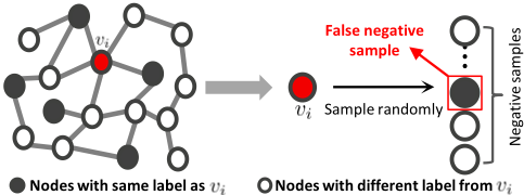
2016] and contrastive methods [Veliˇckovi´c et al., 2019; Hassani and Khasahmadi, 2020]. Among them, the contrastive learning methods, which usually learn representations by leveraging local mutual information maximization across the graph's patch representations, have outperformed even supervised methods and become a prominent technique. However, existing contrastive learning methods fail to consider the class information, leading to less discriminative representations. Meanwhile, as illustrated in Figure 1, these methods usually randomly select negative samples, which would bring false-negative samples with the same class as positive samples. This phenomenon, which we refer to as sampling bias [Chuang et al., 2020], can empirically lead to a significant performance drop.
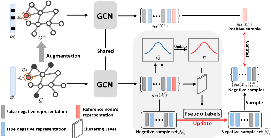
To address the above problems, this paper presents a graph debiased contrastive learning method, which can jointly perform representation learning and clustering in a unified framework. Specifically, we obtain graph representations by contrasting positive and negative pairs. At the same time, we perform a clustering layer to predict their class information with an auxiliary target distribution, which could align the representations with clustering results. In addition, to correct the sampling bias, we randomly select negative samples from the clusters that are different from the positive sample's cluster. By iteratively optimizing the graph representations, the clustering results, and the negative samples on the end-to-end training process, these three parts can benefit from each other.
Our main contributions can be summarized into the following three aspects:
- We propose an end-to-end contrastive learning frame-
- work that can jointly learn graph representations and clustering results from unlabeled graph datasets.
- We develop a debiased sampling strategy to correct the bias for negative samples, where the clustering results are employed to decrease the false-negative samples. Both theoretical analysis and experimental results indicate that, the proposed debiased strategy could alleviate the sampling bias phenomenon.
- Extensive experiments demonstrate that our learned representation is consistently competitive on clustering and classification tasks.
2 RelatedWork
2.1 Unsupervised Graph Representation Learning
Generative Approaches learn representations by designing loss functions in the output space. Among them, most methods use auto-encoder framework to capture the latent representation. Graph Auto-Encoder (GAE) [Kipf and Welling, 2016] first merges GCN [Kipf and Welling, 2017] as an encoder into the auto-encoder framework to seek the latent representation by reconstructing the adjacency matrix. However, GAE fails to consider the data distributions of the latent representation and suffer from inferior embedding in realworld graph data. So, [Pan et al., 2018] enforced the latent codes to match a prior distribution. But the decoder part in these methods cannot be learnable and the graphical feature cannot be used at all in the decoder part. Then, [Park et al., 2019] proposes the first completely symmetric graph convolutional autoencoder, which utilizes both the structure of the graph attributes through the whole encoding-decoding process. Moreover, due to the strong ability of the Generative Adversarial Network (GAN) [Goodfellow et al., 2014] for distribution matching, some works [Pan et al., 2018; Gao et al., 2019; Zheng et al., 2020] have introduced GAN into the unsupervised graph representation learning.
Contrastive Approaches design objective function in latent space by contrasting positive and negative pairs. Deep Graph Infomax (DGI) [Veliˇckovi´c et al., 2019] obtains node representations by maximizing mutual information [Hjelm et al., 2019] between patch representations and corresponding highlevel summaries of graphs. Then, Multi-View Graph Representation Learning method (MVGRL) [Hassani and Khasahmadi, 2020] introduces different structural views into DGI for learning node and graph-level representations. And [You et al., 2020] explored different augmentation strategies to facilitate invariant representation learning.
However, these methods fail to consider the class information, leading to less discriminative representations. And the randomness of negative samples in these methods would lead to a sampling bias problem, resulting in performance decrease. In this paper, we propose a graph debiased contrastive learning framework, where the class information could be predicted by a clustering layer as well as utilized to correct the sampling bias.
2.2 Deep Clustering
Deep clustering approaches [Xie et al., 2016; Ji et al., 2017; Yang et al., 2019; Dang et al., 2020; Yang et al., 2020b] integrate the embedding and clustering processes to obtain optimal embedding subspace for clustering, which can be more effective than shallow clustering methods [Ng et al., 2001; Yang et al., 2018]. For example, Deep Embedding Clustering (DEC) [Xie et al., 2016] learns a mapping from the data space to a lower-dimensional feature space, in which, it iteratively optimizes a clustering objective. To help the auto-encoder learn a better data representation, Improved Deep Embedding Clustering (IDEC) [Guo et al., 2017] adds a reconstruction loss to DEC as a constraint, which can jointly optimize cluster labels assignment and learn features that are suitable for clustering. Then, [Ji et al., 2017] introduced a novel selfexpressive layer between the encoder and decoder to mimic the self-expressiveness property that has proven to be effective in traditional subspace clustering. In addition, to generate discriminative and robust latent representations, [Yang et al., 2019] proposed a novel dual autoencoder network with the mutual information estimation and different reconstruction results.
In this paper, with an auxiliary target distribution, a clustering layer is introduced into our graph contrastive learning framework to make each other optimize better. In addition, aiming to correct the sampling bias, the clustering results could intervene the negative sampling process to decrease the false-negative samples.
3 Method
In this section, we present the proposed graph debiased contrastive learning framework in detail, starting with the overall framework of contrastive objectives, followed by specific graph clustering part. In our framework, the graph contrastive learning and clustering can be optimized jointly and benefit from each other, and the clustering results can alleviate the affect of false-negative samples, correcting the sampling bias in contrastive learning. The whole framework is illustrated in Figure 2.
3.1 ProblemFormulation
We denote an undirected graph as G = {V, E,X}. V = {vi}ni=1 is the finite set of n nodes. E ∈ Rn×n defines the adjacency relationships (i.e., edges) between nodes in G. X ∈ Rn×d records the node features, that is, each node vi is associated with a d-dimensional feature vector xi. According to the adjacency relationships in E, the corresponding adjacent matrix of graph G can be denoted as A ∈ Rn×n , and then we can obtain the diagonal degree matrix D according to Dii = ∑j Aij .
3.2 Graph Contrastive Learning
For simplicity, the graph contrastive learning framework is consist of the commonly used graph convolution network (GCN) [Kipf and Welling, 2017], denoted as gΘ(·). The key idea of graph contrastive learning is to contrast semantically similar (positive) and dissimilar (negative) pairs of data points, encouraging the representation of similar pairs (xi, x+i ) to be close, and those of dissimilar pairs (xi, x-i ) to be more orthogonal:
where the x+i is obtained by utilizing a feature-space augmentation strategy: masking node feature xi randomly, and {x-it }Mt=1 is M negative samples, which is usually randomly selected from V except vi. Note that the graph after this feature-space augmentation is denoted as G+ = {V +, E,X +}, and X + = {x+i }ni=1 records the node features of V +.
However, this framework fails to consider the class information, leading to less discriminative representations. And without access to labels, the randomly sampled negative samples may actually have the same label as the positive sample, causing performance drop. Thus, we introduce a clustering layer into this framework and jointly optimize it with graph representations to alleviate these problems.
3.3 Graph Clustering
We first perform a clustering layer on the embedded representation gΘ(xi) to joint optimize with graph contrastive learning framework. Then, a debiased strategy is developed through clustering layer to decrease the false-negative samples, correcting the sampling bias phenomenon in graph contrastive learning.
Aiming to obtain more accurate clustering results (pseudo labels) and discriminative representations, the clustering loss Lclus is utilized to optimize clustering and contrastive learning simultaneously. And Lclus is defined as the KL divergence is calculated between distributions P and Q, where Q is the distribution of soft labels measured by student's tdistribution and P is the target distribution derived from Q:
where k represents the k-th node in V, j represents the j-th cluster. qkj is the similarity between embedded representation gΘ(xk) and cluster center µj, and qkj is measured by Student's t-distribution:
pkj in Equation 2 is the target distribution P defined as:
And the cluster centers {µj}Cj=1 are initialized by employing clustering layer on gΘ(X), where C represents the number of clusters. Therefore, the loss on the whole framework can be denoted as:
where α is a hyper-parameter that controls the compromise between the two terms. Moreover, in the training process, the target distribution P serves as groundtruth soft label but also depends on predicted soft label. Thus, to avoid instability, P should not be updated at each iteration. In practice, P is updated every T iterations according to Equation 4. And given the learning rate lr, the clusters are updated by the backpropagation:
At the same time, the graph contrastive learning framework's weights are updated by:
In this way, representations can be optimized by aligning with the clustering results, and simultaneously, the optimized representations can promote clustering, leading to more powerful results.
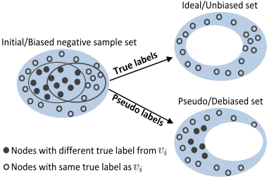
Debiased Strategy. After we obtain the precise clustering results, we can randomly select negative samples from the clusters which are different from the positive samples' cluster. In this way, as the supervisory signals, the clustering results can be utilized to effectively decrease the falsenegative samples in the negative sampling process. Without access of labels, existing graph contrastive learning methods [Veliˇckovi´c et al., 2019; Hassani and Khasahmadi, 2020; You et al., 2020] obtain the negative samples by randomly sampling from the set Ni = {vm}(m ̸= i), which would exist several false-negative samples. As shown in Figure 3, the ideal negative sample set for vi can be obtained when nodes with same true label as vi are removed from Ni. However, since ground-truth labels are unavailable, the pseudo labels is alternatively used to decrease the false-negative samples, which can alleviate the negative effect of false-negative points. Specifically, the pseudo labels generated by the clustering layer are denoted as Yp = {yi}ni=1 . Then, to decrease the false-negative samples in Ni, we remove nodes with the same pseudo label as node vi from Ni, and denote the new negative node set as ˜ Ni:
Algorithm 1 Graph Debiased Contrastive Learning
Input: Graph G, Maximum Iterations MaxIter
Parameter: GCN parameter Θ, hyper-parameter: sample
size of negative points M
Output: Optimized GCN parameters, clustering results.
- 1: Initialize Θ, {µj}Cj=1 according to Section 4.2.
- 2: while iter ∈ {0, 1, ...,MaxIter} do
- 3: if iter%T == 0 then
- 4: Embed node representations by gΘ(·)
- 5: Update P by Equation 4.
- 6: end if
- 7: Generate Yp by clustering layer.
- 8: Update {Ni}ni=1 by Equation 8.
- 9: Update Θ, {µj}Cj=1 by Equation 6 and 7.
- 10: end while
Actually, clustering can also have false predictions, which means the pseudo labels are not exactly accurate. Therefore, ˜ Ni may still have slight false-negative nodes, but it can be proved through a simple mathematical derivation that this debiased strategy could still decrease the false-negative samples to correct the sampling bias.
The whole algorithm is summarized in Algorithm 1. With the joint optimization of GCN and clusters, we could obtain the discriminative representations and clustering results, simultaneously.
4 Experiments
In this section, we first detail our experimental protocol, and then present comparision results of our method with the state of the art for graph representation learning.
4.1 Datasets
For comparison, we select five widely used graph datasets to verify the performance of our method in unsupervised representation learning. Specifically, for node classification and clustering, there are three citation network datasets, i.e., Cora, Citeseer and Pubmed. Moreover, for graph classification, we use two datasets: MUTAG and PTC-MR.
4.2 Experimental Setup
Protocols and EvaluationMetrics. The task of node clustering and node classification are employed to evaluate the learned node representation of contrastive learning. In particular, for node clustering, we adopt the results predicted by clustering layer directly. As in [Park et al., 2019], accuracy (ACC), normalized mutual information (NMI), and adjusted rand index (ARI) are used to measure the performance of clustering. And we report the averaged clustering results over 20 times of execution. While for node classification, we closely follow the experimental setup of DGI [Veliˇckovi´c et al., 2019] and report the mean classification accuracy with standard deviation on the test nodes after 20 runs. Finally, for graph classification, we followMVGRL [Hassani and Khasahmadi, 2020] and report the mean 10-fold cross validation accuracy with standard deviation after 5 runs.
| Method | Cora | Citeseer | Pubmed | ||||||
|---|---|---|---|---|---|---|---|---|---|
| ACC | NMI | ARI | ACC | NMI | ARI | ACC | NMI | ARI | |
| Spectral | 36.7 | 12.6 | 3.1 | 23.8 | 5.5 | 1.0 | 52.8 | 9.7 | 6.2 |
| k-means | 49.2 | 32.1 | 22.9 | 54.0 | 30.5 | 27.8 | 59.5 | 31.5 | 28.1 |
| GAE | 59.6 | 42.9 | 34.7 | 40.8 | 17.6 | 12.4 | 67.2 | 27.7 | 27.9 |
| VGAE | 50.2 | 32.9 | 25.4 | 46.7 | 26.0 | 20.5 | 63.0 | 22.9 | 21.3 |
| DGI | 55.4 | 41.1 | 32.7 | 51.4 | 31.5 | 32.6 | 58.9 | 27.7 | 31.5 |
| ARGA | 64.0 | 44.9 | 35.2 | 57.3 | 35.0 | 34.1 | 66.8 | 30.5 | 29.5 |
| ARVGA | 64.0 | 45.0 | 37.4 | 54.4 | 26.1 | 24.5 | 69.0 | 29.0 | 30.6 |
| MVGRL | 73.2 | 56.2 | 51.9 | 68.1 | 43.2 | 43.4 | 69.3 | 34.4 | 32.3 |
| GALA | 74.5 | 57.6 | 53.1 | 69.3 | 44.1 | 44.6 | 69.3 | 32.7 | 32.1 |
| DBGAN | 74.8 | 56.0 | 54.0 | 67.0 | 40.7 | 41.4 | 69.4 | 32.4 | 32.7 |
| Ours w/o Lclus | 76.4 | 60.9 | 56.2 | 70.2 | 45.8 | 46.0 | 71.0 | 35.6 | 34.2 |
| Ours | 78.1 | 61.0 | 57.9 | 71.9 | 46.4 | 46.9 | 72.0 | 36.5 | 34.6 |
| Methods | Cora | Citeseer | Pubmed |
|---|---|---|---|
| Ours w/o PL &Lclus | 72.8 | 67.2 | 68.0 |
| Ours w/o PL | 74.8 | 69.9 | 70.8 |
| Ours w/o Lclus | 76.4 | 70.2 | 71.0 |
| Ours | 78.1 | 71.9 | 72.0 |
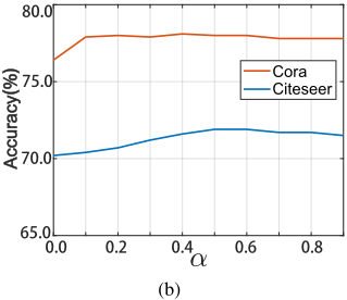
ImplementationDetails. Following suggestions in [Guo et al., 2017], we pretrain the contrastive learning framework before perform debiased strategy. And the cluster centers {µj}Cj=1 are initialized by employing clustering layer on gΘ(X). For node clustering task, one-layer GCN is used in the graph contrastive framework and the hidden dimension of GCN is set to 220. The learning rate is set to 0.0001 on Cora and Citeseer, 0.00004 on Pubmed. The hyper-parameter α is set to 0.1 on Cora and Pubmed, 0.5 on Citeseer. For the node classification task, the learning rate is set to 0.01 on all three datasets when optimize the classification layer. For the graph classification task, the hidden dimension of GCN is 512, α is set to 0.3 on MUTAG and PTC-MR datasets.
4.3 Node Clustering
Comparison Methods. We compare our method with two kinds of clustering methods: I. methods that only use features or graph structures: k-means and DeepWalk [Perozzi et al., 2014]; II. methods that use both features and graph structures: Spectral clustering, GAE [Kipf and Welling, 2016], VGAE [Kipf and Welling, 2016], ARGA [Pan et al., 2018], ARVGA [Pan et al., 2018]. DGI [Veliˇckovi´c et al., 2019], MVGRL [Hassani and Khasahmadi, 2020], GALA [Park et al., 2019] and DBGAN [Zheng et al., 2020].
Results Analysis. Table 1 depicts the clustering performance with three different metrics on Cora, Citeseer and Pubmed datasets. It shows that we could achieve remarkable performance on all three datasets. For example, we achieve 78.1%, 71.9% and 72.0% accuracy on Cora, Citeseer and Pubmed datasets, which have 3.3%, 2.6% and 1.9% relative improvement over previous state-of-the art, respectively. We can observe that without the clustering loss, it also can outperform the state-of-the art, e.g., 76.4% vs 74.8% on Cora dataset, which indicate that the proposed debiased strategy is effective. Moreover, these compared methods usually first learn representations, and then the learned representations are clustered by k-means or spectral clustering [Park et al., 2019; Zheng et al., 2020]. Meanwhile, our end-to-end model can obtain better embedded representations and clustering results, simultaneously. In addition, existing graph contrastive approaches DGI [Veliˇckovi´c et al., 2019] and MVGRL [Hassani and Khasahmadi, 2020] use two-layer GCN with 512 hidden dimension while one-layer GCN with 220 hidden dimension is used in our model. Therefore, we have fewer parameters of model while our proposed method outperform them. Moreover, the ablation study has been done as shown in Table 2. Without the clustering loss, our method with the debiased strategy also outperforms the basic graph contrastive learning framework, e.g., 76.4% vs 72.8% on Cora dataset, which indicates that the pseudo labels can actually correct the sampling bias.
| Methods | Cora | Citeseer | Pubmed |
|---|---|---|---|
| DeepWalk | 70.7± 0.6 | 51.4±0.5 | 74.3±0.9 |
| GAE | 71.5±0.4 | 65.8±0.4 | 72.1±0.5 |
| GCN | 81.5±0.3 | 70.3±0.4 | 79.0±0.3 |
| GAT | 83.0±0.7 | 72.5±0.7 | 79.0±0.3 |
| DeepGCN | 85.5±0.3 | 73.4±0.4 | 80.3±0.5 |
| DGI | 83.8±0.5 | 72.0±0.6 | 77.9±0.3 |
| MVGRL | 86.8±0.5 | 73.3±0.5 | 80.1±0.7 |
| Ours w/o PL | 86.5±0.4 | 73.3±0.3 | 80.0±0.8 |
| Ours w/o Lclus | 87.0±0.6 | 73.8±0.5 | 80.6±0.4 |
| Ours | 87.8±0.5 | 74.5±0.6 | 81.0 ±0.5 |
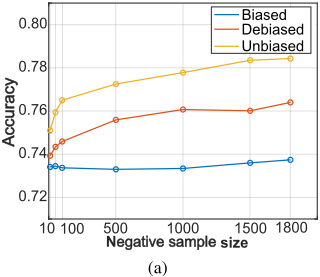
Parameter Analysis. And as depicted in Figure 4(a), we explore the influence of negative sample size (M) to our model on Cora dataset. To better explore the influence, we remove the clustering loss, so the clustering accuracy curves with/without debiased strategy are reported. For comparison, we also record the accuracy curve of the graph contrastive learning framework with unbiased negative sampling. The negative sample size barely have affect on the biased contrastive learning, which is mainly caused by the existence of false-negative samples. On the contrary, the accuracy of both unbiased and debiased contrastive learning improve gradually with the increase of the negative sample size. Compared to the unbiased contrastive learning, accuracy of the biased is lower, indicating that the sampling bias would lead to performance dropping. Furthermore, the parameter sensitivity analysis of α on node clustering are depicted in Figure 4(b).
4.4 Node Classification
Comparison Methods. To evaluate node classification under the linear evaluation protocol, we compare our method with unsupervised methods including DeepWalk [Perozzi et al., 2014], GAE [Kipf and Welling, 2016], DGI [Veliˇckovi´c et al., 2019] and MVGRL [Hassani and Khasahmadi, 2020]. Moreover, we compare our results with supervised models including GCN [Kipf and Welling, 2017], GAT [Veliˇckovi´c et al., 2018] and DeepGCN [Chen et al., 2020].
Results Analysis. The results reported in Table 3 show that we achieve state-of-the art results with respect previous unsupervised model and even supervised GNN methods. More specifically, we can achieve better accuracy than the state-ofthe art method MVGRL [Hassani and Khasahmadi, 2020], e.g., , 87.8% vs 86.8% on Cora dataset and 81.0% vs 80.1% on Pubmed dataset. These results demonstrate that our graph contrastive learning framework could learn more discriminative representations under the assistance of clustering layer.
| Methods | MUTAG | PTC-MR |
|---|---|---|
| RandomWalk node2vec graph2vec infoGraph MVGRL Ours | 83.7± 1.5 72.6±10.2 83.2±9.6 89.0±1.1 89.7±1.1 90.5±1.6 | 57.9±1.3 58.6±8.0 60.2±6.9 61.7±1.4 62.5±1.7 63.6±1.8 |
4.5 Graph Classification
Our model can also perform the graph-level contrastive learning. When we learn representations on graph level, we need to add a readout layer to the GCN output of each graph. Correspondingly, the inputs of the clustering layer are the readout outputs of multiple graphs, and the sampling process is also for graphs.
Comparison Methods. We compare the results with five unsupervised methods including Random Walk [G¨artner et al., 2003], node2vec [Grover and Leskovec, 2016], graph2vec [Narayanan et al., 2017], InfoGraph [Sun et al., 2020] and MVGRL [Hassani and Khasahmadi, 2020].
Results Analysis. The results shown in Table 4 suggest that our approach achieves state-of-the-art results with respect to unsupervised models. It shows that we could achieve remarkable performance on both datasets. For example, we achieve 90.5%, 63.6% accuracy on MUTAG and PTC-MR datasets, which have 0.8% and 1.1% relative improvement over previous state-of-the art method MVGRL.
5 Conclusion
In this paper, we design a graph debiased contrastive learning model, which jointly performs graph representation learning and clustering in a unified framework. With an auxiliary target distribution, the graph representations and clustering results are jointly optimized to obtain better results. At the same time, aiming to correct the sampling bias in the negative samples, the clustering results are utilized to decrease the false-negative samples. Extensive experiments demonstrate that the representation and clusters learned by our method is consistently competitive on graph classification, node clustering and classification tasks.
Acknowledgments
Our work was supported in part by the National Natural Science Foundation of China under Grant 62071361, and in part by the Fundamental Research Funds for the Central Universities ZDRC2102.
@inproceedings{ijcai2021p473,
  title     = {Graph Debiased Contrastive Learning with Joint Representation Clustering},
  author    = {Zhao, Han and Yang, Xu and Wang, Zhenru and Yang, Erkun and Deng, Cheng},
  booktitle = {Proceedings of the Thirtieth International Joint Conference on
               Artificial Intelligence, {IJCAI-21}},
  publisher = {International Joint Conferences on Artificial Intelligence Organization},
  editor    = {Zhi-Hua Zhou},
  pages     = {3434--3440},
  year      = {2021},
  month     = {8},
  note      = {Main Track},
  doi       = {10.24963/ijcai.2021/473},
  url       = {https://doi.org/10.24963/ijcai.2021/473},
}
TY - CPAPER TI - Graph Debiased Contrastive Learning with Joint Representation Clustering AU - Zhao, Han AU - Yang, Xu AU - Wang, Zhenru AU - Yang, Erkun AU - Deng, Cheng T2 - Proceedings of the Thirtieth International Joint Conference on Artificial Intelligence, IJCAI-21 PB - International Joint Conferences on Artificial Intelligence Organization PY - 2021 SP - 3434 EP - 3440 DO - 10.24963/ijcai.2021/473 UR - https://doi.org/10.24963/ijcai.2021/473 ER -Copied
Machine-readable versions of this paper, for tools and AI agents:





