
Eliminating the Computation of Strongly Connected Components in Generalized Arc Consistency Algorithm for AllDifferent Constraint
Proceedings of the Thirty-Second International Joint Conference on Artificial Intelligence. Main Track. Pages 2049-2057.
https://doi.org/10.24963/ijcai.2023/228
Keywords
- Constraint Satisfaction and Optimization: CSO: Constraint satisfaction
- Constraint Satisfaction and Optimization: CSO: Constraint programming
Abstract
AllDifferent constraint is widely used in Constraint Programming to model real world problems. Existing Generalized Arc Consistency (GAC) algorithms map an AllDifferent constraint onto a bipartite graph and utilize the structure of Strongly Connected Components (SCCs) in the graph to filter values. Calculating SCCs is time-consuming in the existing algorithms, so we propose a novel GAC algorithm for AllDifferent constraint in this paper, which eliminates the computation of SCCs. We prove that all redundant edges in the bipartite graph point to some alternating cycles. Our algorithm exploits this property and uses a more efficient method to filter values, which is based on breadth-first search. Experimental results on the XCSP3 benchmark suite show that our algorithm considerably outperforms the state-of-the-art GAC algorithms.
- [Berge, 1973] Claude Berge. Graphs and hypergraphs. American Elsevier Publishing Company, 1973.
- [Bessiere and Régin, 1997] Christian Bessiere and Jean- Charles Régin. Arc consistency for general constraint net- works: preliminary results. In IJCAI, volume 2, pages 398-404.
- [Bessiere et al., 2004] Christian Bessiere, Emmanuel He- brard, Brahim Hnich, and Toby Walsh. Disjoint, partition and intersection constraints for set and multiset variables. CP, 4:138-152, 2004.
- [Boussemart et al., 2004] Frédéric Boussemart, Fred Hemery, Christophe Lecoutre, and Lakhdar Sais. Boost- ing systematic search by weighting constraints. In ECAI, volume 16, page 146, 2004.
- [Boussemart et al., 2016] Frédéric Boussemart, Christophe Lecoutre, Gilles Audemard, and Cédric Piette. Xcsp3: an integrated format for benchmarking combinatorial con- strained problems. arXiv preprint arXiv:1611.03398, 2016.
- [Bundy and Wallen, 1984] Alan Bundy and Lincoln Wallen. Breadth-first search. In Catalogue of artificial intelligence tools, pages 13-13. Springer, 1984.
- [Fellows et al., 2013] Michael Fellows, Tobias Friedrich, Danny Hermelin, Nina Narodytska, and Frances Rosa- mond. Constraint satisfaction problems: Convexity makes alldifferent constraints tractable. Theoretical Computer Science, 472:81-89, 2013.
- [Gent et al., 2008] Ian P Gent, Ian Miguel, and Peter Nightingale. Generalised arc consistency for the alldif- ferent constraint: An empirical survey. AI, 172(18):1973- 2000, 2008.
- [Jean-Charles, 1996] Régin Jean-Charles. Generalized arc consistency for global cardinality constraint. American Association for Artificial Intelligence (AAAI 1996), pages 209-215, 1996.
- [Kuhn, 1955] Harold W Kuhn. The hungarian method for the assignment problem. Naval research logistics quarterly, 2(1-2):83-97, 1955.
- [Lauriere, 1978] Jena-Lonis Lauriere. A language and a pro- gram for stating and solving combinatorial problems. AI, 10(1):29-127, 1978.
- [López-Ortiz et al., 2003] Alejandro López-Ortiz, Claude- Guy Quimper, John Tromp, and Peter Van Beek. A fast and simple algorithm for bounds consistency of the alld- ifferent constraint. In IJCAI, volume 3, pages 245-250, 2003. IJCAI
- [Prud'homme et al., 2016] Charles Prud'homme, Jean- Guillaume Fages, and Xavier Lorca. Choco solver documentation. TASC, INRIA Rennes, LINA CNRS UMR, 6241, 2016.
- [Puget, 1998] Jean-Franc ¸ois Puget. A fast algorithm for the bound consistency of alldiff constraints. In AAAI, pages 359-366, 1998.
- [Régin, 1994] Jean-Charles Régin. A filtering algorithm for constraints of difference in csps. In AAAI, volume 94, pages 362-367, 1994.
- [Rossi et al., 2006] Francesca Rossi, Peter Van Beek, and Toby Walsh. Handbook of constraint programming. El- sevier, 2006.
- [Shaw, 2004] Paul Shaw. A constraint for bin packing. In Principles and Practice of Constraint Programming-CP 2004: 10th International Conference, CP 2004, Toronto, Canada, September 27-October 1, 2004. Proceedings 10, pages 648-662. Springer, 2004.
- [Suijlen et al., 2022] Wijnand Suijlen, Félix de Framond, Arnaud Lallouet, and Antoine Petitet. A parallel algorithm for gac filtering of the alldifferent constraint. In Interna- tional Conference on Integration of Constraint Program- ming, Artificial Intelligence, and Operations Research, pages 390-407. Springer, 2022.
- [Tardivo et al., 2022] Fabio Tardivo, Agostino Dovier, An- drea Formisano, Laurent Michel, and Enrico Pontelli. Constraints propagation on gpu: A case study for alldif- ferent. In PCILC, CEUR-WS, 2022.
- [Tarjan, 1972] Robert Tarjan. Depth-first search and linear graph algorithms. SIAM journal on computing, 1(2):146- 160, 1972,.
- [Van Hoeve et al., 2006] Willem-Jan Van Hoeve, Gilles Pe- sant, Louis-Martin Rousseau, and Ashish Sabharwal. Re- visiting the sequence constraint. In Principles and Prac- tice of Constraint Programming-CP 2006: 12th Interna- tional Conference, CP 2006, Nantes, France, September 25-29, 2006. Proceedings 12, pages 620-634. Springer, 2006.
- [Van Hoeve, 2001] Willem-Jan Van Hoeve. The alldifferent constraint: A survey. arXiv preprint cs/0105015, 2001.
- [Van Kessel and Quimper, 2012] Philippe Van Kessel and Claude-Guy Quimper. Filtering algorithms based on the word-ram model. In AAAI, volume 26, pages 577-583, 2012.
- [Wallace, 1996] Mark Wallace. Practical applications of constraint programming. Constraints, 1(1):139-168, 1996.
- [Zhang et al., 2018] Xizhe Zhang, Qian Li, and Weixiong Zhang. A fast algorithm for generalized arc consistency of the alldifferent constraint. In IJCAI, pages 1398-1403, 2018. IJCAI
- [Zhang et al., 2020] Xizhe Zhang, Jian Gao, Yizhi Lv, and Weixiong Zhang. Early and efficient identification of use- less constraint propagation for alldifferent constraints. In IJCAI, pages 1126-1133, 2020. IJCAI
References were extracted automatically from the PDF and may contain errors.
Full text extracted automatically from the PDF; figures, tables and equations may differ. The PDF is the version of record.
1 Introduction
Constraint Programming (CP) is a powerful paradigm for solving combinatorial search problems [Rossi et al., 2006]. When solving problems with CP, people model the real world problem into a Constraint Satisfaction Problem (CSP) defined with a set of variables whose values must satisfy some constraints. Then a general purpose constraint solver is used to solve the CSP. AllDifferent constraint (hereinafter, called allDiff ) [Lauriere, 1978] requires that the values of the variables in this constraint must be different. Because of its practical interests, allDiff has been widely used in modelling many real world problems in CP [Wallace, 1996; Van Hoeve, 2001; Fellows et al., 2013].
A solution to a CSP is an assignment to all variables that satisfies all constraints. Solving a CSP involves either finding a solution or proving that there is no solution to the CSP. Backtracking search is a standard algorithm for solving CSPs. To speedup the search process, local consistency techniques are used to filter out some inconsistent values from the domains of the variables. Generalized Arc Consistency (GAC) [Bessiere and R´egin, 1997] is one of the most popular local consistencies in modern constraint solvers. A classical GAC algorithm of allDiff was proposed by R´egin [R´egin, 1994]. It maps an allDiff to a value graph and filters values by removing redundant edges that do not appear in any maximum matching of the value graph. To avoid enumerating all maximum matchings, the algorithm identifies all Strongly Connected Components (SCCs) of the value graph and removes edges between the SCCs. In 2008, Gent et al. proposed an algorithm [Gent et al., 2008] capturing all SCCs of the value graph and updating the local part of the value graph. In 2018, Zhang et al. proposed an algorithm [Zhang et al., 2018] that improves R´egin's algorithm by finding SCCs on subgraphs of value graphs. In 2020, Zhang et al. proposed a mechanism for early detection of useless propagations [Zhang et al., 2020]. In recent years, some other approaches have emerged, such as using GPU [Tardivo et al., 2022] or parallel algorithms [Suijlen et al., 2022] to maintain the consistency of allDiff.
The computation of SCCs [Tarjan, 1972] is the basis of the existing GAC algorithms of allDiff. However, the computation is time-consuming in the GAC algorithms. Computing all SCCs is rather time-consuming in R´egin's algorithm [R´egin, 1994]. Although Gent's algorithm [Gent et al., 2008] uses an incremental updating strategy to compute SCCs, it take a considerable amount of time to maintain all the SCC information. Zhang's 2018 algorithm proves that the computation of SCCs in subgraphs of the value graph is sufficient to enforce GAC and it is several times faster than R´egin's algorithm. In Zhang's 2020 algorithm [Zhang et al., 2020], a preprocessing algorithm is inserted to avoid unnecessary computation of SCCs and it further saves some computation time in solving some problems. Based on the aforementioned analysis, the solving time will be significantly reduced if the computation of SCCs is eliminated from the GAC algorithm for allDiff.
In this paper, we propose a novel GAC algorithm for allDiff that eliminates the computation of SCCs. We first define Reachable Set (RS), a set of vertices, in the value graph of allDiff. Then we prove that any edge whose ending vertex is in an RS and starting vertex is out of the RS is redundant. Based on our new finding, we design an efficient GAC algorithm that filters values by calculating RSs. In the first run, our algorithm calculates the RSs for all variables in the constraint. After that, we recalculate the RSs only for the variables whose domains have been changed.
Extensive experiments have been performed on the XCSP3 benchmark suite [Boussemart et al., 2016]. The results show that our algorithm outperforms the state-of-the-art algorithms in solving most of the problems containing allDiff. In the problems where the number of allDiff s accounts for a large proportion of the total number of constraints, such as Karuro, QWH, etc., our algorithm performs significantly better than the existing algorithms. We believe that our algorithm could be a new component for modern constraint solvers to handle allDiff.
2 Background
A constraint satisfaction problem (CSP) P is a triple P = ⟨X,D, C⟩, where X is a set of n variables X = {x1, x2, · · · , xn}, D is a set of domains D = {D(x1), D(x2), · · · , D(xn)}, where D(xi) is a finite set of possible values for variable xi, and C is a set of e constraints C = {c1, c2, · · · , ce}. Each constraint c consists of two parts, an ordered set of variables scp(c) = {xi1, xi2, · · · , xir} and a subset of the Cartesian product D(xi1) × D(xi2) × · · · × D(xir) that specifies the allowed (or disallowed) combinations of values for the variables {xi1, xi2, · · · , xir}. An element of D(xi1) × D(xi2) × · · · × D(xir) is called a tuple on scp(c), denoted by τ. τ[x] is the value of x in τ. A tuple τ is valid for a constraint c iff ∀xi ∈ scp(c), τ[xi] ∈ D(xi), otherwise τ is invalid.
A solution to a CSP is an assignment of values to each variable such that all constraints in the CSP are satisfied. Solving a CSP P involves either finding one (or more) solution(s) of P or proving that P is unsatisfiable. Backtracking search is a standard algorithm for solving CSPs. It performs a depthfirst traversal of a search tree. At each search tree node, an unassigned variable is selected and a new node is generated after the assignment to this variable, and then constraint propagation is applied to filter those inconsistent values from the domains of variables. If the propagation leads a domain to be wiped out, then a failure is encountered, one or more assignments must be cancelled and a backtracking occurs.
Constraint propagation establishes local consistency in CSP to filter invalid values. Generalized Arc Consistency (GAC) [Bessiere and R´egin, 1997] is one of the most important local consistencies in constraint solvers, which is defined as follows.
Definition 1 (Generalized Arc Consistency). Given a CSP P = ⟨X , D, C⟩, a constraint c ∈ C, and a variable x ∈ scp(c),
- A value x = a is consistent with c iff there exists a valid tuple τ allowed by c and τ[x] = a.
- Constraint c is generalized arc consistent iff ∀ x ∈ scp(c), D(x) ̸= ∅ and ∀ a ∈ D(x), x = a is consistent with c.
- P is generalized arc consistent iff all the constraints of C are generalized arc consistent.
An allDiff c requires that the values of the variables in this constraint must be different. The relations between the variables in scp(c) and the values in the domains of the variables can be represented by a value graph which is a specific case of directed bipartite graph defined as follows.
Definition 2 (Value Graph). Given an allDiff c, the value graph of c is a bipartite graph ⟨U, V, E⟩, where U = scp(c), V = ⋃u∈U D(u), E = {(u, v)|u ∈ U, v ∈ D(u)} and |E| = ∑u∈U |D(u)|.
An edge (u, v) implies that its direction is from u to v. A matching in a graph is a set of edges without common vertices. An edge is a matching edge if it is in the matching; otherwise it is a non-matching edge. A vertex is called a matching vertex if it is related to an edge in the matching, otherwise a free vertex. A path is a finite sequence of edges which joins a sequence of vertices, a directed path is a path whose edges are all directed in same direction. A vertex u can reach a vertex v if there exists a directed path from u to v. An alternating path is a path whose edges are alternately in and out of the matching. An augmenting path is an alternating path whose starting and ending vertices are free vertices. A cycle is a directed path which starts and ends at the same vertex. An alternating cycle is a cycle whose edges are alternately in and out of the matching, a single vertex that is not contained in an even alternating cycle or an even alternating path ending at a free vertex can also be called an alternating cycle. A maximum matching is a matching with the maximum number of edges. In a value graph, a maximum matching is a matching with the edge number equals to min(|U|, |V |), which can be computed by the Hungarian algorithm [Kuhn, 1955]. Example 1 illustrates the value graph of an allDiff where the set of red edges is a maximum matching.
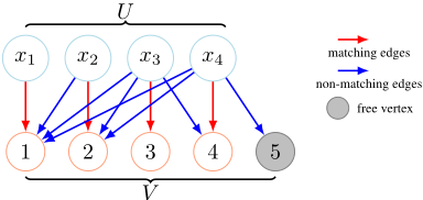
Example 1. Given an allDiff c1, where scp(c1) = {x1, x2, x3, x4}, D(x1) = {1}, D(x2) = {1, 2}, D(x3) = {1, 2, 3, 4}, D(x4) = {1, 2, 4, 5}. The value graph of c1 is shown in Figure 1.
V
Figure 1: The value graph for allDiff c1 in Example 1.
Amaximummatching of a value graph of allDiff is a valid tuple, so an edge in the value graph is a redundant one if it does not belong to any maximum matching. An allDiff satisfies GAC iff all edges in its value graph are non-redundant. However, it is quite time-consuming to enumerate all maximum matchings, so the existing GAC algorithms for allDiff identify redundant edges based on the following theorem [Berge, 1973].
Theorem 1. For an arbitrary maximum matching, a nonmatching edge in the value graph is allowed iff it belongs to either an even alternating path ending at a free vertex or an even alternating cycle.
Existing GAC algorithms for allDiff map an allDiff onto a value graph. To identify redundant edges, these algorithms find a maximum matching of the value graph and reverse all edges in the matching, and then find even alternating paths ending at free vertices and even alternating cycles based on the computation of SCCs.
3 RelatedWork
We recall some classical and efficient GAC algorithms for allDiff here. In 1994, R´egin proposed a GAC algorithm [R´egin, 1994] for allDiff, which is considered as the basis of the existing GAC algorithms. It finds a maximum matching in the value graph and reverses all matching edges. Then a virtual vertex t is added into the value graph. After that, it adds edges from free vertices to t and edges from t to the matching vertices in V of the graph. Finally, it computes all SCCs of the graph and removes edges between SCCs.
In 2008, Gent et al. proposed a method that avoids the computation of unchanged SCCs [Gent et al., 2008]. It maintains the information of each SCC in the value graph and only checks the SCCs containing the variables whose domains have been changed between successive propagations. Thus, it recomputes only the affected SCCs and removes the edges between SCCs. By reducing the computation of SCCs, it is more efficient than R´egin's algorithm in solving some problems.
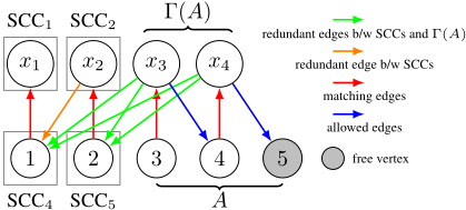
In 2018, Zhang et al. proposed an efficient algorithm (hereinafter, called Zhang18 algorithm) based on R´egin's algorithm [Zhang et al., 2018]. It improves R´egin's algorithm by finding SCCs in a sub-graph of the value graph. In their algorithm, some redundant edges can be obtained by finding alternating paths ending at free vertices. More specifically, it identifies the set A containing all the vertices in V that can reach free vertices and the set Γ(A) containing all the vertices in U that can reach free vertices. Then, each edge starting at a vertex in Γ(A) and ending at a vertex in V \A is redundant. The remaining redundant edges can be found by computing SCCs in the induced subgraph of (U \Γ(A))∪(V \A). Note that Zhang18 algorithm degenerates to R´egin's algorithm if there is no free vertex in the value graph. Figure 2 shows the value graph of Zhang18 algorithm for c1 in Example 1. The green edges in Figure 2 are identified by finding alternating paths, and the orange edge is identified by computing SCCs.
In 2020, Zhang et al. proposed a new algorithm [Zhang et al., 2020] (hereinafter, called Zhang20 algorithm) that identifies useless propagations. The algorithm considers an edge to be unimportant if there exists an alternating cycle in the graph containing the end nodes of the edge after removing it. They proved that the removal of an unimportant edge does not need to invoke constraint propagation. Zhang20 algorithm brings improvements in solving some problems.
Among some modern constraint solvers, the Ace solver 1 and the Minion solver 2 chose Gent's algorithm as the GAC algorithm for allDiff, the Choco solver 3 [Prud'homme et al., 2016] chooses R´egin's algorithm and Zhang18 algorithm as the GAC algorithm for allDiff. Zhang20 algorithm has not yet been implemented in mainstream constraint solvers. In addition to GAC, Bound Consistency (BC) [Puget, 1998; L´opezOrtiz et al., 2003] is also used in modern constraint solvers as a consistency used by propagation algorithms for allDiff. In general, BC is less capable of deleting values than GAC. In addition to the above algorithms, a method [Van Kessel and Quimper, 2012] based on bitwise operations was proposed by Kessel and Quimper in 2012, however, their method is rarely used in modern constraint solvers.
4 Eliminating the Computation of SCCs
Computing SCCs in a value graph is time-consuming, thus the propagation time of allDiff will be significantly reduced if the computation of SCCs is eliminated. To discuss the properties of redundant edges, we first introduce two notions. An even alternating cycle is called an EAC and an even alternating path ending at a free vertex is called an EAPF.
Corollary 1. For an arbitrary maximum matching, a nonmatching edge in the value graph is redundant, iff it belongs to neither an EAPF nor an EAC.
Corollary 1 is the contrapositive of Theorem 1. By Corollary 1, we know that every redundant edge is either between an EAPF and an EAC, or between two EACs. Note that there is no redundant edge between two EAPFs, because such an edge connects two EAPFs and results in a longer EAPF.
Corollary 2. Given two EACs C1 and C2, V (C1) and V (C2) are the vertex sets of C1 and C2 respectively. All the redundant edges between V (C1) and V (C2) are directed either exclusively from the vertices in V (C1) to the vertices in V (C2) or exclusively from the vertices in V (C2) to the vertices in V (C1).
Proof. Assuming that there exists a redundant edge directed from a vertex in V (C1) to a vertex in V (C2) and a redundant edge directed from a vertex in V (C2) to a vertex in V (C1), then there exists another EAC which is a supergraph of C1 and C2. However, by Corollary 1, redundant edges do not belong to any EAC. There exists a contradiction. Thus, the corollary is proven.
Corollary 3. Given an EAPF P1 and an EAC C1, V (P1) and V (C1) are their vertex sets respectively. All the redundant edges between V (P1) and V (C1) are directed from the vertices in V (P1) to the vertices in V (C1).
1 https://github.com/xcsp3team/ace
2 https://constraintmodelling.org/minion/
3 https://choco-solver.org/
Proof. Assuming that there exists a redundant edge e directed from a vertex in V (C1) to a vertex in V (P1), then e belongs to an EAPF. However by Theorem 1, e is an allowed edge. This is in contradiction with the precondition that e is a redundant edge. Thus, the corollary is proven.
Corollary 4. Every redundant edge ends at a vertex in an EAC and starts at a vertex out of the EAC it ends in.
By Corollary 2 and 3, we can conclude Corollary 4. If we can find all EACs containing the end vertices of all redundant edges, then all redundant edges can be obtained. Therefore, it is not necessary to find all EACs.
Definition 3 (Reachable Set). Given a variable x, and mx is the starting vertex of the matching edge (mx, x), the reachable set RS(x) is the set of vertices reachable frommx.
For each variable x, RS(x) can be computed by BreadthFirst Search (BFS) starting from the vertex mx with worstcase time complexity of O(|E| + |V | + |U|) [Bundy and Wallen, 1984]. Example 2 shows the RSs of some variables.
Example 2. Given an allDiff c2, where scp(c2) = {x1, x2, x3, x4, x5}, D(x1) = {1}, D(x2) = {1, 2}, D(x3) = {3, 4}, D(x4) = {3, 4}, D(x5) = {3, 4, 5}. The value graph of c2 is shown in Figure 3, RS(x1) = {1, x1}, and RS(x4) = {4, x4, 3, x3}.
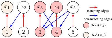
By Definition 3, if there is only one value in the domain of the variable x, then mx can only reach the vertex x, because the only value in D(x) is in the matching and the edge is from the value to x. In this case, RS(x) = {mx, x} because mx is not contained in an EAC or an EAPF, mx is considered as an EAC.
Theorem 2. Given an RS(x) containing no free vertex and two vertices u, v in the value graph, u ̸∈ RS(x) and v ∈ RS(x). If there exists an edge (u, v), then the edge (u, v) is redundant.
Proof. By Definition 3, given v ∈ RS(x) and u ̸∈ RS(x), v can not reach u, so there is no EAC containing (u, v). Since RS(x) contains no free vertex and v ∈ RS(x), v can not reach any free vertex, so there exists no EAPF containing (u, v). By Corollary 1, (u, v) is redundant.
Theorem 2 provides us an efficient idea to identify redundant edges in a value graph. We propose an efficient GAC algorithm for allDiff that eliminates the computation of SCCs in Algorithm 1. The main idea is to compute RSs for each variable then to remove all the edges directed to the vertices in the RSs containing no free vertex.
Algorithm 1 filtering algorithm for allDiff
Require: allDiff c
1: construct the value graph G = ⟨U, V,E⟩ for c; 2: XD ← {x | x ∈ scp(c) and |D(x)| ̸= lastSize(c)[x]}; 3: for all x ∈ XD do 4: if the matching edge for x does not exist then 5: if repair matching edges for x fails then 6: return inconsistency; 7: M ← the maximummatching; 8: for all x ∈ XD do 9: XD ←XD \ {x}; 10: compute RS(x); 11: if RS(x) contains a free vertex then 12: continue; 13: for all v ∈ RS(x) do 14: if the edge (u, v) exists and u ̸∈ RS(x) then 15: remove (u, v) fromG; 16: D(u) ← D(u) \ {v}; 17: XD ← XD ∪ {u}; 18: for all x ∈ scp(c) do 19: lastSize(c)[x] ← |D(x)|;For each allDiff c, we use G to store the value graph and a backtrackable array lastSize(c) to store the domain sizes of the variables in scp(c). There are two ways to implement the value graph G, one is to reconstruct G from c when Algorithm 1 is called, and the other is to use decremental backtrackable data structures to store G. And Algorithm 1 uses the latter. For each variable x ∈ scp(c), lastSize(c)[x] records the domain size of x. The domain size is used to obtain the variables whose domains have been changed since the last time c was processed. Each lastSize(c)[x] of each allDiff c is initialized to 0, so at the beginning of the search, all variables in scp(c) are added into XD at line 2, which is a set containing the variables to be processed. After that, we compare the current domain size of each variable x with its recorded domain size. If the number |D(x)| is not equal to the number lastSize(c)[x], then D(x) has been changed since the previous invocation of Algorithm 1 for the specific constraint c and x will be added into XD .
At lines 3-6, we use an incremental strategy to find new matching edges for the variables in XD whose matching edges are removed. At the beginning of the search, the Hungarian algorithm [Kuhn, 1955] is employed to find a maximum matching. After that, if the matching edge for x is removed, the new matching edge for x can be found by the augmenting path. If there is no maximum matching, i.e. the matching edge for a variable can not be repaired, then there is no valid tuple, by Definition 1, c does not satisfy GAC and the inconsistency is returned at line 6.
The redundant edges are removed at lines 8-17. The variables in XD are selected and removed from the set and processed one by one. For each variable x selected from XD , we compute RS(x) with BFS. If RS(x) contains a free vertex, we skip the variable x; otherwise, any edge directed from a vertex u /∈ RS(x) to a vertex v ∈ RS(x) is deleted. The RS(x) containing a free vertex is skipped at line 12, because the redundant edges directed to a vertex in RS(x) will be processed later. The reason for this is as follows: If all vertices in RS(x) can reach a free vertex, then all the edges directed to a vertex in RS are contained in an EAPF, so there are allowed edges; otherwise, there exists a vertex v in RS(x) that can not reach a free vertex. In the latter case, there exists a vertex u′ involved in the matching edge (v, u′ ) (otherwise, v is a free vertex), so v belongs to RS(u′ ). RS(u′ ) contains no free vertex, because v in RS(x) can not reach a free vertex. When processing RS(u′ ), the redundant edges directed to v will be deleted. Example 3 illustrates the case. If an edge is removed during the procedure, the related variables will be added into XD at line 17. Finally, the domain sizes of the variables in scp(c) are recorded in lastSize(c).
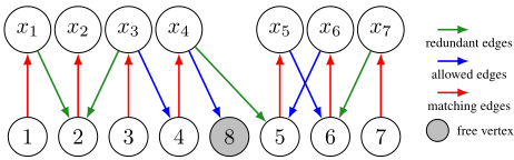
Example 3. Given an allDiff c3, where scp(c3) = {x1, x2, x3, x4, x5, x6, x7}, D(x1) = {1, 2}, D(x2) = {2}, D(x3) = {2, 3, 4}, D(x4) = {4, 5, 8}, D(x5) = {5, 6}, D(x6) = {5, 6}, D(x7) = {6, 7}, the value graph of c3 is shown in Figure 4. When processing RS(x3) = {x2, x3, x4, x5, x6, 2, 3, 4, 5, 6, 8}, the redundant edges (x1, 2) and (x7, 6) are not deleted because RS(x3) contains free vertex 8. The vertex 6 and vertex 2 belong to RS(x6) and RS(x2) respectively. The two RSs contain no free vertex, so the redundant edges (x4, 5), (x7, 6) and (x1, 2), (x3, 2) will be deleted when processing the two RSs.
The worst-case time complexity of Algorithm 1 is O(|scp(c)|*(|E| + |V | + |U|)). Although the time complexity of BFS for computing RS and Tarjan's algorithm for computing SCCs [Tarjan, 1972] are both O(|E| + |V | + |U|), performing BFS for RS is more efficient than performing Tarjan's algorithm for SCCs in the realistically implementations of the GAC algorithms for allDiff.
Example 4 and 5 describe the processing of two allDiff s by Algorithm 1. Example 4 describes the case when nonmatching edges are deleted from the value graph of c4 and Example 5 describes the case when the matching edge is deleted from the value graph of c5.
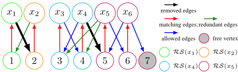
Example 4. Given an allDiff c4, where scp(c4) = {x1, x2, x3, x4, x5, x6}, D(x1) = {1, 2}, D(x2) = {1, 2}, D(x3) = {3, 4}, D(x4) = {3, 4, 5}, D(x5) = {3, 4, 5, 6}, D(x6) = {5, 6, 7}, the value graph of c4 is shown in Figure 5. When the value 2 is removed from D(x1) and the value 5 is removed from D(x4) by the solver, the black dashed lines represent the edge (x1, 2) and (x4, 5) that are removed. Algorithm 1 processes c4 as follows:
b. x1 ∈ XD , get RS(x1), RS(x1) = {1, x1}.
- 1 ∈RS(x1), and x2 ̸∈RS(x1), remove the edge (x2, 1), D(x2) = D(x2) \ {1}, XD = {x2, x4}.
d. x2 ∈ XD , get RS(x2), RS(x2) = {2, x2}, do nothing.
- x4 ∈ XD , get RS(x4), RS(x4) = {4, x4, 3, x3}.
- 3, 4 ∈ RS(x4), and x5 ̸∈ RS(x4), remove the edge (x5, 3) and (x5, 4), D(x5) = D(x5) \ {3, 4}, XD = {x5}.
- x5 ∈XD , get RS(x5), RS(x5) = {5, x5, 6, x6, 7}.
h. RS(x5) contains a free vertex, do nothing.
- XD = ∅, Algorithm 1 ends.
Example 5. Given an allDiff c5, where scp(c5) = {x1, x2, x3, x4}, D(x1) = {1, 2}, D(x2) = {2, 3}, D(x3) = {3, 4}, D(x4) = {1, 4}, the value graph of c5 is shown in Figure 6(a). When the value 1 is removed from D(x1) by the solver. First, Algorithm 1 repairs a new matching edge for x1 by finding an augmenting path (x1, 2, x2, 3, x3, 4, x4, 1), and the new matching is shown in Figure 6(b). Then, Algorithm 1 computes RS(x1) and deletes (x2, 2), and then computes RS(x2), RS(x3) and RS(x4) in turn. Finally, D(x1) = {2}, D(x2) = {3}, D(x3) = {4}, D(x4) = {1}.
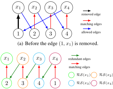
- (b) After repairing a new matching edge for x1.
Figure 6: The value graphs of allDiff c5 in Example 5.
Theorem 3. There is no allowed edge removed by Algorithm 1.
Proof. The ending vertex and starting vertex in each edge removed by Algorithm 1 are not in the same RS. By Theorem 2, all edges directed to a vertex in an RS not containing a free vertex is redundant. Thus, Algorithm 1 does not remove any allowed edge.
Theorem 4. Algorithm 1 removes all redundant edges.
Proof. In the first run of Algorithm 1 for a allDiff c, all variables in scp(c) will be added into XD and their RSs will be processed at lines 8-17. For each redundant edge (u, v), by Corollary 4, v belongs to an EAC and u cannot be reached by any vertex in the EAC. Let x be the ending vertex of the matching edge (v, x), then x is a vertex in the EAC, so RS(x) does not contain u. When processing RS(x) at lines 13-17, the edge (u, v) will be deleted, because u does not belong to RS(x) and v belongs to RS(x).
Whenever the domain of a variable u is changed during propagation, u is added into XD at line 17. Assuming that the value v is removed from D(u), which leads to the deletion of the edge (u, v) from the value graph. If there exists an redundant edge (u′ , v′ ) after the deletion, then u can not reach u′ . This is because if u can reach u′ , then RS(u) contains u′ and v′ , so there exists an EAC containing u, u′ and v′ , and (u′ , v′ ) is an allowed edge. In this way, when processing RS(u), the redundant edge (u′ , v′ ) will be deleted. Therefore, all redundant edges are removed by Algorithm 1.
Amaximummatching of a value graph of allDiff is a valid tuple, so an edge in the value graph is a redundant one if it does not belong to any maximum matching. By Definition 1, an allDiff satisfies GAC iff all edges in its value graph are non-redundant. Therefore, removing all the redundant edges in the value graph is equivalent to making the corresponding allDiff satisfy GAC. By Theorem 3 and 4, Algorithm 1 only removes all redundant edges in the value graph of allDiff c, so Algorithm 1 makes the allDiff c satisfy GAC.
5 Experimental Results
In order to show the practical interest of our GAC algorithm, we conducted experiments using a Windows 10 PC with an AMD Ryzen 3950X processor and 64 GB memory. To prevent the effects of CPU overclocking, the CPU clock speed was fixed at 3.7GHz and the CPU warm-up process was performed before all experiments were conducted. The Java Development Kit version is openjdk-18.0.1.1.
We compared our algorithm with four efficient GAC algorithms including R´egin's algorithm [R´egin, 1994], Gent's algorithm [Gent et al., 2008], Zhang18 algorithm [Zhang et al., 2018] and Zhang20 algorithm [Zhang et al., 2020]. We used Choco solver [Prud'homme et al., 2016] in the experiment. R´egin's algorithm and Zhang18 algorithm have been already integrated in the solver, so we implemented our algorithm, Gent's algorithm and Zhang20 algorithm. The source code of our algorithm is available here 4 . The performance of finding the first solution and proving unsatisfable is measured by CPU time in seconds. The timeout limit is set to 900 seconds.
The experiments were run with the XCSP3 benchmark suite 5 , which contains 21 families of CSP instances defined by at least one allDiff. After eliminating the instances where all algorithms are timeout, 1285 instances were involved in the experiments 6 .
4 https://github.com/luhanzhen/AllDifferent
5 http://www.xcsp.org
10 -2 10 -1 10 0 10 1 10 2 10 3
Our algorithm(s)
10 -2 10 -1 10 0 10 1 10 2 10 3
Our algorithm(s)
10 -2 10 -1 10 0 10 1 10 2 10 3
Our algorithm(s)
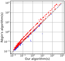
Figure 7: Comparing our algorithm with the existing GAC algorithms by pairs.
We used a deterministic variable ordering heuristic called min lower bound first (hereinafter, called minLB), which always selects the variable with the smallest domain size (the leftmost variable has higher priority). The heuristic called lower bound value first was always selected as the value ordering heuristic. With these low-cost heuristics, the search with all the compared GAC algorithms build the same search tree for each CSP instance, so we can examine the improvement measured by solving time of our propagation algorithm and others.
In Figure 7, we compare our GAC algorithm with the existing algorithms by pairs. The X-axis of the scatter plots is the time cost (seconds) of our algorithm and the Y-axis is the time cost (seconds) of the existing algorithms. The red scatters above the diagonals represent the instances where our algorithm performs better and the blue ones under rhe diagonals represent the instances where the other algorithms perform better. More specifically, the numbers of red scatters to that of blue scatters in the four sub-figures are (1128:147), (1133:142), (976:301) and (1207:65) respectively. It is observed that our algorithm outperforms the other algorithms.
In Table 1, we report the average solving time cost for solving these problems. The best one in each row is in bold. It can be seen that our algorithm achieves the best performance in 18 out of 21 problems. It brings a significant improve-
6 The Subisomorphism problem contains a large number of instances, so we selected 2 sub-problems with 300 instances in our experiments.
Zhang18 algorithm(s)
10 3
10 2
10 1
10 0
10 -1
10 -2
Gent's algorithm(s)
Zhang20 algorithm(s)
10 3
10 2
10 1
10 0
10 -1
10 -2
10 3
10 2
10 1
10 0
10 -1
10 -2
| Series | #Instances | R´egin | Gent | Zhang18 | Zhang20 | Our |
|---|---|---|---|---|---|---|
| AllInterval | 14 | 54.69 | 51.74 | 54.77 | 66.14 | 44.16 |
| ColouredQueens | 5 | 0.10 | 0.11 | 0.09 | 0.11 | 0.05 |
| CostasArray | 9 | 153.26 | 157.98 | 118.28 | 191.80 | 52.59 |
| CoveringArray | 2 | 0.018 | 0.019 | 0.018 | 0.018 | 0.016 |
| CryptoPuzzle | 10 | 0.020 | 0.020 | 0.020 | 0.020 | 0.018 |
| DeBruijnSequence | 7 | 0.130 | 0.139 | 0.133 | 0.164 | 1.491 |
| Kakuro | 538 | 12.72 | 12.95 | 11.34 | 13.23 | 7.53 |
| KnightTour | 10 | 49.57 | 46.24 | 49.69 | 53.65 | 37.24 |
| Langford | 15 | 13.96 | 13.16 | 13.92 | 16.52 | 11.83 |
| QWH | 37 | 229.00 | 216.11 | 228.39 | 263.28 | 128.91 |
| BQWH | 198 | 0.019 | 0.020 | 0.018 | 0.020 | 0.018 |
| MagicSquare | 18 | 5.05 | 4.60 | 4.93 | 6.32 | 5.71 |
| nengfa | 3 | 5.59 | 5.23 | 4.09 | 7.40 | 3.81 |
| NumberPartitioning | 25 | 85.22 | 77.74 | 81.64 | 98.71 | 66.42 |
| Ortholatin | 5 | 17.35 | 16.61 | 17.39 | 20.31 | 7.45 |
| QuasiGroups | 23 | 42.04 | 48.63 | 46.53 | 44.58 | 40.90 |
| Queens | 12 | 28.81 | 30.28 | 30.11 | 31.77 | 30.01 |
| SchurrLemma-mod | 6 | 88.30 | 95.50 | 60.97 | 138.09 | 37.76 |
| SportsScheduling | 2 | 0.018 | 0.019 | 0.018 | 0.019 | 0.018 |
| Subisomorphism | 300 | 2.55 | 2.51 | 2.49 | 2.48 | 2.19 |
| Sudoku | 46 | 0.015 | 0.016 | 0.015 | 0.016 | 0.016 |
| Instances | #Constraints | #allDiff | R´egin | Gent | Zhang18 | Zhang20 | Our |
|---|---|---|---|---|---|---|---|
| AllInterval-019 | 56 | 2 | 653.55 | 613.76 | 653.55 | 791.17 | 528.83 |
| CostasArray-17 | 149 | 15 | 748.71 | 770.16 | 576.36 | >900 | 258.24 |
| CostasArray-18 | 167 | 16 | 545.54 | 562.84 | 421.44 | 715.36 | 184.51 |
| Kakuro-easy-168 | 532 | 266 | >900 | >900 | 836.18 | >900 | 477.93 |
| Kakuro-medium-181 | 536 | 268 | 458.60 | 492.32 | 309.46 | 529.33 | 156.78 |
| Kakuro-hard-168 | 168 | 84 | 30.39 | 32.69 | 21.04 | 34.88 | 10.71 |
| Kakuro-hard-178 | 540 | 270 | >900 | >900 | >900 | >900 | 648.02 |
| qwh-o30-h375-04 | 61 | 60 | 661.64 | 601.68 | 704.19 | >900 | 246.24 |
| qwh-o100-h10000 | 200 | 200 | 241.90 | 230.53 | 261.07 | 266.37 | 104.29 |
| Mixed-nengfa-protein X2 | 569 | 1 | 16.64 | 15.56 | 12.13 | 22.03 | 10.73 |
| KnightTour-08 | 66 | 1 | 494.55 | 461.29 | 495.73 | 535.29 | 371.52 |
| Langford-2-13 | 14 | 1 | 208.46 | 196.48 | 207.87 | 246.75 | 176.49 |
| NumberPartitioning-084 | 92 | 1 | 263.10 | 229.91 | 248.76 | 308.04 | 195.00 |
| Ortholatin-007 | 80 | 29 | 86.67 | 82.97 | 86.91 | 101.50 | 37.19 |
| QuasiGroup-4-08 | 129 | 16 | 92.05 | 89.31 | 87.67 | 90.87 | 59.95 |
| SchurrLemma-100-9 | 2450 | 2450 | 341.33 | 383.59 | 246.29 | 569.55 | 159.37 |
| Subisomorphism-si2-r01-m200-08 | 158 | 1 | 606.34 | 570.29 | 570.58 | 581.93 | 470.91 |
| Subisomorphism-si4-r01-m200-02 | 581 | 1 | 873.33 | 859.68 | 839.07 | 884.42 | 794.21 |
| DeBruijnSequence-02-08 | 2051 | 1 | 0.65 | 0.70 | 0.66 | 0.85 | 9.67 |
ment in some problems, such as CostasArray, QWH, Ortholatin, SchurrLemma-mod, etc. However, for a family of CSP instances called DeBruijnSequence, our algorithm is not as good as the others, the reason is that our algorithm is very inefficient for three instances within this family, and this can be observed from the blue scatters that deviate to the right of the diagonals in Figure 7.
In Table 2, we present the results of some representative instances, together with the numbers of constraints in these instances. Compared with the existing algorithms, our algorithm saves more CPU time in the instances where the number of allDiff accounts for a large proportion of the total number of constraints. For example, if we consider Zhang18 algorithm as a baseline, our algorithm saves about 12% to
19% CPU time in Mixed-nengfa-protein X2 and AllInterval019. Moreover, it saves about 35% to 65% CPU time in SchurrLemma-100-9 and qwh-o30-h375-04. We can conclude that the improvement in efficiency of our algorithm for a given instance is positively correlated with the number of allDiff constraints as a proportion of all constraints in that instance, further demonstrating the significant improvement of our algorithm over the other four algorithms.
Nevertheless, we can observe from the last row of Table 2 that our algorithm is much less efficient than the other four algorithms. The reason for this situation is that for the instance named DeBruijnSequence-02-08, there is an allDiff constraint with 256 variables whose domains are from 0 to 255, there is a situation where some vertices are computed multiple times in RSs, or even a situation where one RS contains most of the vertices of the value graph.
The reasons why our algorithm is more efficient than the other four algorithms are as follows: Compared with R´egin's algorithm and Zhang18 algorithm, our algorithm updates the value graph locally and eliminates the computation of SCCs. Compared with Gent's algorithm, our algorithm not only eliminates the task of recording information about the SCCs in the value graph, but also the value graph in our algorithm does not contain the virtual vertex. Compared with Zhang20 algorithm, our algorithm does not require the solver to record all deleted edges, and it does not spend time checking whether unimportant edges exist. Therefore, our algorithm removes all redundant edges in the value graph at a much lower cost.
10 -2 10 -1 10 0 10 1 10 2 10 3
Our algorithm(s)
10 -2 10 -1 10 0 10 1 10 2 10 3
Our algorithm(s)
10 -2 10 -1 10 0 10 1 10 2 10 3
Our algorithm(s)
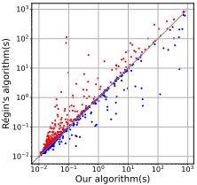
Figure 8: Comparing our algorithm with the existing GAC algorithms by pairs with dom/wdeg heuristic.
We have compared the solving efficiency of the GAC algorithms with the low-cost variable ordering heuristic which builds the same search trees. Then, we examined the per-
Zhang18 algorithm(s)
10 3
10 2
10 1
10 0
10 -1
10 -2
Gent's algorithm(s)
Zhang20 algorithm(s)
10 3
10 2
10 1
10 0
10 -1
10 -2
10 3
10 2
10 1
10 0
10 -1
10 -2
formance of the GAC algorithms when using a more efficient variable ordering heuristic dom/wdeg [Boussemart et al., 2004]. Since the Choco solver may process different variables with empty domains in the same scope at dom/wdeg in different order, this heuristic can lead to distinct search trees under distinct filtering algorithms. The result is shown in Figure 8. Specifically, the number of red scatters to that of blue scatters in the four sub-figures are (833:442), (919:354), (699:576) and (875:399) respectively. Although the dom/wdeg heuristic has an unpredictable effect on the path of the backtracking search, we observe that our algorithm still outperforms the existing algorithms. The reason for this phenomena is that our algorithm consumes less time to enforce GAC for allDiff compared with other existing algorithms.
6 Conclusion
In this paper, we propose a novel GAC algorithm for allDiff. Our algorithm eliminates the computation of SCCs, which is time-consuming in existing GAC algorithms for allDiff. Instead of computing the SCCs, our algorithm uses a simpler and more efficient method called BFS to identify redundant edges. The experimental results on the XCSP3 benchmark suite show that our algorithm outperforms four efficient GAC algorithms for allDiff. It not only brings significant improvement in the problems where the number of allDiff is a large proportion of the total number of constraints, but also indirectly improves the propagation algorithms for other constraints (e.g. Global Cardinality Constraint [Jean-Charles, 1996], Sequence Constraint [Van Hoeve et al., 2006], Disjoint Constraint [Bessiere et al., 2004], Bin Packing Constraint [Shaw, 2004], etc.). The new algorithm could be a new candidate propagator for allDiff inmodern constraint solvers.
Acknowledgements
The authors would like to thank the anonymous reviewers for their helpful comments. This work is supported by the National Natural Science Foundation of China under Grant 62276060, the Natural Science Foundation of Jilin Province under Grant 20210101470JC, and the Industrial Technology Research and Development Project of the Development and Reform Commission of Jilin Province 2019C053-9.
@inproceedings{ijcai2023p228,
  title     = {Eliminating the Computation of Strongly Connected Components in Generalized Arc Consistency Algorithm for AllDifferent Constraint},
  author    = {Zhen, Luhan and Li, Zhanshan and Li, Yanzhi and Li, Hongbo},
  booktitle = {Proceedings of the Thirty-Second International Joint Conference on
               Artificial Intelligence, {IJCAI-23}},
  publisher = {International Joint Conferences on Artificial Intelligence Organization},
  editor    = {Edith Elkind},
  pages     = {2049--2057},
  year      = {2023},
  month     = {8},
  note      = {Main Track},
  doi       = {10.24963/ijcai.2023/228},
  url       = {https://doi.org/10.24963/ijcai.2023/228},
}
TY - CPAPER TI - Eliminating the Computation of Strongly Connected Components in Generalized Arc Consistency Algorithm for AllDifferent Constraint AU - Zhen, Luhan AU - Li, Zhanshan AU - Li, Yanzhi AU - Li, Hongbo T2 - Proceedings of the Thirty-Second International Joint Conference on Artificial Intelligence, IJCAI-23 PB - International Joint Conferences on Artificial Intelligence Organization PY - 2023 SP - 2049 EP - 2057 DO - 10.24963/ijcai.2023/228 UR - https://doi.org/10.24963/ijcai.2023/228 ER -Copied
Machine-readable versions of this paper, for tools and AI agents:





