
Model Checking Causality
Proceedings of the Thirty-Third International Joint Conference on Artificial Intelligence. Main Track. Pages 3324-3332.
https://doi.org/10.24963/ijcai.2024/368
Keywords
- Knowledge Representation and Reasoning: KRR: Causality
- Knowledge Representation and Reasoning: KRR: Knowledge representation languages
Abstract
We present a novel modal language for causal reasoning and interpret it by means of a semantics in which causal information is represented using causal bases in propositional form. The language includes modal operators of conditional causal necessity where the condition is a causal change operation. We provide a succinct formulation of model checking for our language and a model checking procedure based on a polysize reduction to QBF. We illustrate the expressiveness of our language through some examples and show that it allows us to represent and to formally verify a variety of concepts studied in the field of explainable AI including abductive explanation, intervention and actual cause.
- [Audemard et al., 2020] Gilles Audemard, Frédéric Koriche, and Pierre Marquis. On tractable XAI queries based on compiled representations. In Proceedings of the 17th In- ternational Conference on Principles of Knowledge Repre- sentation and Reasoning (KR 2020), pages 838-849, 2020.
- [Beckers, 2021a] Sander Beckers. Causal sufficiency and actual causation. Journal of Philosophical Logic, 50(6):1341-1374, 2021.
- [Beckers, 2021b] Sander Beckers. The counterfactual NESS definition of causation. In Proceedings of the Thirty- Fifth AAAI Conference on Artificial Intelligence (AAAI- 21), pages 6210-6217. AAAI Press, 2021.
- [Belnap et al., 2001] Nuel Belnap, Michael Perloff, and Ming Xu. Facing the future: agents and choices in our indeterminist world. Oxford University Press, New York, 2001.
- [Burks, 1951] Arthur W. Burks. The logic of causal proposi- tions. Mind, 60(239):363-382, 1951.
- [Cooper and Marques-Silva, 2023] Martin C. Cooper and João Marques-Silva. Tractability of explaining classifier decisions. Artificial Intelligence, 316:103841, 2023.
- [Darwiche and Hirth, 2020] Adnan Darwiche and Auguste Hirth. On the reasons behind decisions. In Proceedings of the 24th European Conference on Artificial Intelligence (ECAI 2020), volume 325 of Frontiers in Artificial Intelli- gence and Applications, pages 712-720. IOS Press, 2020.
- [Eiter and Lukasiewicz, 2002] Thomas Eiter and Thomas Lukasiewicz. Complexity results for structure-based causality. Artificial Intelligence, 142(1):53-89, 2002. IJCAI
- [Galles and Pearl, 1998] David Galles and Judea Pearl. An axiomatic characterization of causal counterfactuals. Foundation of Science, 3(1):151-182, 1998.
- [Gattinger, 2023] Malvin Gattinger. HasCacBDD, 2023. Version 0.1.0.4, Feb. 3, 2023.
- [Gladyshev et al., 2023] Maksim Gladyshev, Natasha Alechina, Mehdi Dastani, Dragan Doder, and Brian Logan. Dynamic causality. In Proceedings of the 26th European Conference on Artificial Intelligence (ECAI 2023), volume 372 of Frontiers in Artificial Intelligence and Applications, pages 867-874. IOS Press, 2023.
- [Halpern and Pearl, 2001] Joseph Y. Halpern and Judea Pearl. Causes and explanations: A structural-model ap- proach: Part 1: Causes. In Proceedings of the 17th Con- ference in Uncertainty in Artificial Intelligence (UAI '01), pages 194-202.
- Morgan Kaufmann, 2001. [Halpern and Pearl, 2005a] Joseph Y. Halpern and Judea Pearl. Causes and explanations: a structural-model ap- proach. Part I: Causes. British Journal for Philosophy of Science, 56(4):843-887, 2005.
- [Halpern and Pearl, 2005b] Joseph Y. Halpern and Judea Pearl. Causes and explanations: a structural-model ap- proach. Part II: Explanations. British Journal for Philoso- phy of Science, 56(4):889-911, 2005.
- [Halpern, 2000] Joseph Y. Halpern. Axiomatizing causal reasoning. Journal of Artificial Intelligence Research, 12:317-337, 2000.
- [Halpern, 2008] Joseph Y. Halpern. Defaults and normality in causal structures. In Gerhard Brewka and Jérôme Lang, editors, Principles of Knowledge Representation and Rea- soning: Proceedings of the Eleventh International Confer- ence (KR 2008), pages 198-208. AAAI Press, 2008.
- [Halpern, 2015] Joseph Y. Halpern. A modification of the Halpern-Pearl definition of causality. In Proceedings of the Twenty-Fourth International Joint Conference on Artificial Intelligence (IJCAI 2015), pages 3022-3033. AAAI Press, 2015. IJCAI
- [Halpern, 2016] Joseph Y. Halpern. Actual causality. MIT Press, 2016.
- [Ignatiev et al., 2019] Alexey Ignatiev, Nina Narodytska, and João Marques-Silva. Abduction-based explanations for machine learning models. In Proceedings of the Thirty- third AAAI Conference on Artificial Intelligence (AAAI- 19), volume 33, pages 1511-1519, 2019.
- [Izza and Marques-Silva, 2021] Yacine Izza and João Marques-Silva. On explaining random forests with SAT. In Zhi-Hua Zhou, editor, Proceedings of the Thirtieth International Joint Conference on Artificial Intelligence (IJCAI 2021), pages 2584-2591. ijcai.org, 2021. IJCAI
- [Liu and Lorini, 2022] Xinghan Liu and Emiliano Lorini. A logic of "black box" classifier systems. In Proceedings of the 28th International Workshop on Logic, Language, Information, and Computation (WOLLIC 2022), volume 13468 of LNCS, pages 158-174. Springer, 2022.
- [Liu and Lorini, 2023] Xinghan Liu and Emiliano Lorini. A unified logical framework for explanations in classifier systems. Journal of Logic and Computation, 33(2):485- 515, 2023.
- [Lorini, 2019] Emiliano Lorini. Exploiting belief bases for building rich epistemic structures. In Proceedings of the Seventeenth Conference on Theoretical Aspects of Ra- tionality and Knowledge (TARK 2019), volume 297 of EPTCS, pages 332-353, 2019.
- [Lorini, 2020] Emiliano Lorini. Rethinking epistemic logic with belief bases. Artificial Intelligence, 282, 2020.
- [Lorini, 2023] Emiliano Lorini. A rule-based modal view of causal reasoning. In Proceedings of the Thirty-Second In- ternational Joint Conference on Artificial Intelligence (IJ- CAI 2023), pages 3286-3295. ijcai.org, 2023. IJCAI
- [Marques-Silva et al., 2020] João Marques-Silva, Thomas Gerspacher, Martin C. Cooper, Alexey Ignatiev, and Nina Narodytska. Explaining naive bayes and other linear clas- sifiers with polynomial time and delay. In Advances in Neural Information Processing Systems 33: Annual Con- ference on Neural Information Processing Systems 2020, NeurIPS 2020, 2020.
- [Marquis, 1991] Pierre Marquis. Extending abduction from propositional to first-order logic. In Procedings of the In- ternational Workshop on Fundamentals of Artificial Intel- ligence Research (FAIR'91), volume 535 of LNCS, pages 141-155. Springer, 1991.
- [Miller, 2021] Tim Miller. Contrastive explanation: a structural-model approach. The Knowledge Engineering Review, 36:e14, 2021.
- [Shih et al., 2018] Andy Shih, Arthur Choi, and Adnan Dar- wiche. A symbolic approach to explaining bayesian net- work classifiers. In Proceedings of the Twenty-Seventh In- ternational Joint Conference on Artificial Intelligence (IJ- CAI 2018), pages 5103-5111. ijcai.org, 2018. IJCAI
- [van Benthem et al., 2018] Johan van Benthem, Jan van Ei- jck, Malvin Gattinger, and Kaile Su. Symbolic model checking for dynamic epistemic logic -S5 and beyond. Journal of Logic and Computation, 28(2):367-402, 2018.
- [Zhang, 2013] Jiji Zhang. A Lewisian logic of causal coun- terfactuals. Minds and Machines, 23(1):77-93, 2013.
References were extracted automatically from the PDF and may contain errors.
Full text extracted automatically from the PDF; figures, tables and equations may differ. The PDF is the version of record.
1 Introduction
Reasoning about causality plays a pivotal role in AI nowadays given the relevance of causal properties and concepts for explainable AI (XAI). At a mere conceptual level, an explanation can be seen as a causal attribution, namely, as the recognition that a fact F1 (the explanandum) is true because another fact F2 (the explanans) is true. For example, explaining the decision of a classifier system such as a decision tree, a random forest or an artificial neural network (ANN) just consists in recognizing that the classifier made a certain classification because some input features/variables had certain values. Most formal analyses of explanation reduce the problem of checking whether F1 holds because of F2 to the problem checking whether F2 is a sufficient condition (or cause) of F1. They often include the requirement that F2 should be minimal (i.e., no other F ′2 strictly implied by F2 is sufficient for F1). 1 Different notions of explanation and cause based on sufficiency have been formalized. These include sufficient reason [Darwiche and Hirth, 2020] first introduced under the name PI-explanation in [Shih et al., 2018] and also called abductive explanation in [Ignatiev et al., 2019] following previous work on abduction [Marquis, 1991]; sufficient cause and actual cause [Halpern and Pearl, 2005a]; sufficient contrastive cause [Miller, 2021]; NESS (Necessary Element of a Sufficient Set) cause [Beckers, 2021b; Halpern, 2008]; direct/weak/strong sufficiency [Beckers, 2021a].
1 Some formal analyses of explanation also consider the explainer's uncertainty about the values of some variables and/or about the causal model and define explanation relative to the explainer's epistemic state (see, e.g., [Halpern and Pearl, 2005b; Miller, 2021; Liu and Lorini, 2022] or [Halpern, 2016, Chapter 3]).
Some of these notions rely on prime implicant (PI), while the others rely on causal intervention (CI). We call the PIfamily the former and the CI-family the latter. Ignatiev et al.'s abductive explanation (AXp) and Darwiche & Hirth's sufficient reason are representative of the PI-family, while Halpern & Pearl (H&P)'s sufficient cause and actual cause are representative of the CI-family. Complexity analyses for notions in the CI-family, actual cause in particular, can be found in [Eiter and Lukasiewicz, 2002; Gladyshev et al., 2023]. The complexity analysis for the PI-family, especially for abductive explanation, is much richer and depends on the models to be explained ranging from tractable cases such as monotone or linear classifiers [Marques-Silva et al., 2020; Cooper and Marques-Silva, 2023; Audemard et al., 2020] to intractable ones such as random forests [Izza and MarquesSilva, 2021].
Greater attention has been paid by logicians to the CIfamily. In particular, several modal languages of interventionist conditionals [Galles and Pearl, 1998; Halpern, 2000; Halpern and Pearl, 2005a; Zhang, 2013] have been proposed in the recent years that are particularly suited to expressing sufficiency-based notions of explanation and cause belonging to the CI-family. At the semantic level, they are interpreted by means of so-called structural equation models (SEMs). Less attention has been paid by logicians to the PI-family.
In the present paper we rebalance the analysis by introducing a novel modal language and semantics for causal reasoning i) which are general enough to handle notions of explanation and cause from both families, and ii) which are wellsuited for formal verification. We consider ii) an essential requirement given the urgent need to develop theoretically well-founded algorithmic solutions for XAI applications.
Following [Lorini, 2023], at the semantic level we represent causal information using causal bases in propositional form. The idea of replacing relational Kripke models with knowledge bases, of which causal bases are a special case, was also applied to epistemic logic in [Lorini, 2020]. Our semantics has a greater generality than the SEM semantics for at least two reasons. First of all, unlike SEMs, in our semantics there is no rigid distinction between endogenous and exogenous variables which is fixed at the meta-level. Secondly, in our semantics causal information is not necessarily represented in equational form. Thus, we can represent incomplete information about the underlying causal model. However, one can restrict to equational causal bases which guarantee complete information about the causal model and from which exogenous and endogenous variables as well as causal graphs can be extracted.
Using these semantics we interpret a modal language whose main constituent is a concept of conditional causal necessity where the condition is a causal change operation (causal necessity after a certain causal change operation has taken place). An interesting aspect of the language is its modularity. We will show that the special case of conditional causal necessity (causal necessity under no causal change) is captured by a standard S5-modality and is sufficient to capture the notion of abductive explanation belonging to the PIfamily. We will moreover show that to capture H&P's notion of actual cause belonging to the CI-family, one has to condition causal necessity to causal operations corresponding to interventions.
The paper is organized as follows. In Section 2 we introduce our semantics and modal language. In Section 3 we show how to use the language to represent causal notions including abductive explanation, causal necessity post intervention and H&P's actual cause. In Section 4 we present a model checking algorithm for our language based on a polysize reduction to QBF. We illustrate its implementation on an example by providing some experimental results on computation time.
2 Logical Framework
In this section, we present our logical framework for causal reasoning. We first present its semantics in which states in a model include causal information represented in propositional form. Then, we introduce our causal language and interpret it using the semantics. The novel aspect of our language is a new family of conditional causal necessity operators that generalize the S5-modal operator of (unconditional) causal necessity presented in [Lorini, 2023]. 2 Finally, we consider a subclass of states, so-called equational states, in which causal information is represented in equational form. Equational states are needed to be able to relate our analysis of actual cause to H&P's analysis based on structural equational models (SEMs).
2.1 Semantics
Let P be a infinite countable set of atomic propositions whose elements are noted p, q, . . . We note LPROP the propositional language built from P. Elements of LPROP are noted ω, ω′ , . . . Given ω ∈ LPROP, we note with P(ω) the set of atomic propositions occurring in ω. Moreover, if X ⊆ LPROP then P(X) = ⋃ω∈X P(ω).
2 The idea of using the basic modal logic S5 for modeling causal necessity traces back to [Burks, 1951].
The following definition introduces the concept of state, namely, a causal base supplemented with a propositional valuation that is compatible with it.
Definition 1 (State). A state is a pair S = (C, V ), where C ⊆ LPROP is a causal base, and V ⊆ P is a valuation such that ∀ω ∈ C, V |= ω. The set of all states is noted S. A state S = (C, V ) is said to be finite if both C and V are finite.
The valuation V represents the actual environment (or situation), while C represents the base of causal information (viz. the causal base). It is assumed that the former is compatible with the latter, that is, if ω is included in the actual causal base (i.e., ω ∈ C) then it should be true in the actual environment (i.e., V |= ω). The following example illustrates the notion of state.
Example 1. There is a group of agents J = {1, . . . , n} with n > 2 who are writing a paper together. Two solutions are taken into consideration: submitting the paper to a prestigious conference (co), or to a small workshop with no published proceedings (¬co). Each agent i in J can invest either a large (lt i) or a small (¬lt i) amount of time in the collaboration. Whether the paper will be readable (re) or not (¬re) and of high (hq) or low (¬hq) quality depends on how much time the agents invest in the collaboration. Moreover, whether the paper will be accepted (ac) depends on its quality, readility and to which event is submitted. In particular, the actual causal base C0 includes the following four pieces information: i) the paper will be of high quality if and only if at least two agents in the group invest a large amount of time in the collaboration, ii) the paper will be readable if and only if at least one agent in the group invests a large amount of time in the collaboration, iii) if the paper is submitted to the prestigious conference then it will be accepted only if it is of high quality, iv) if the paper is submitted to the small workshop then it will be accepted if and only if it is readable. Thus, there is incomplete information about the underlying causal model: a non-deterministic component is involved since high quality is not a guarantee of acceptance at a prestigious conference. That is, C0 = {ω1, ω2, ω3, ω4} with
We suppose in the current situation only the first agent invests a large amount of time in the collaboration. Moreover, the resulting paper turns out to be readable. It is submitted to the small workshop and is accepted. That is,
It is easy to verify that the valuation V0 is compatible with the information of the causal base C0, i.e., V0 |= ωk for every k ∈ {1, . . . , 4}. Thus, S0 = (C0, V0) is a state.
Let symbols +X and -X denote, respectively, the operation of expanding a causal base with the set of propositional formulas X ⊆ LPROP and the operation of retracting the set of propositional formulas X ⊆ LPROP from a causal base. We call them atomic causal change operations, or simply atomic operations. We note O the set of (possibly empty) sequences of atomic operations and π, π′ , . . . its elements. We note ⋏ the empty sequence. Elements of O are generically called causal change operations, or simply operations.
The following definition introduces the concept of conditional causal compatibility, namely, compatibility between two states conditioned on a certain causal change operation.
Definition 2 (Causal compatibility relation). Let π ∈ O and S = (C, V ), S′ = (C ′ , V ′ ) ∈ S. Then, SRπS′ if and only if C ′ = C π where C π is defined by induction on π:
Note that causal compatibility between two states S and S′ does not depend on their valuations V and V ′ . SRπS′ means that state S′ is causally compatible with state S conditionally on the operation π (or after the operation π has taken place).
Let us go back to Example 1 to illustrate the causal compatibility relation.
Example 2 (cont.). The operation
with ω5 def= ¬co → (hq ↔ ac) replaces the causal rule ω4 with the more demanding rule ω5 which restricts acceptance at the workshop to high quality papers. We have that S0Rπ0 S1 with S1 = (C1, V1) such that C1 = {ω1, ω2, ω3, ω5} and V1 = ∅. This means that state S1 is causally compatible with state S0 conditionally on the causal change operation π0.
2.2 Languages
The following definition introduces our modal language for causal reasoning.
Definition 3 (Language). We structure the language in two layers:
where p ranges over P, ω ranges over LPROP and π ranges over O.
Operators ⊤, ⊥, ∨, → and ↔ are defined as usual abbreviations. The dual of □π is defined, as usual, as ♢π φ def= ¬□π ¬φ.
We call LCI the language of causal information and LCICN the language of causal information and conditional (causal) necessity.
Formula △ω has to be read "the information ω is in the actual causal base", while formula □π φ has to be read "it is causally necessary that φ conditional on the causal change operation π" or "if the causal change operation π occurred, it would be causally necessary that φ". The operator □⋏ is the operator of unconditional causal necessity, namely, causal necessity relative to the actual causal base (when no causal change operation takes place). It was already presented in [Lorini, 2023]. For notational convenience, we abbreviate □φ def= □⋏φ.
For notational convenience, we define the set of atomic formulas:
The following definition of model is needed to provide a semantic interpretation of LCICN-formulas.
Definition 4 (Model). A model is a pair (S, U) such that S ∈ U ⊆ S. The set of models is noted M.
The component U is called context (or universe) of interpretation.
The following definition introduces the satisfaction relation between models and formulas of the language LCICN. (We omit semantic interpretations for the Boolean connectives ¬, ∧ and for ⊤ since they are defined in the usual way.)
Definition 5 (Satisfaction relation). Let (S,U) ∈ M with S = (C, V ). Then,
Note that U in Definition 4 can be any (possibly infinite) set of states with no restriction on the information that is included in a causal base. Nonetheless, in some cases it is useful to restrict to models in which causal bases are constructed from a finite repository of relevant information Γ ⊆ LPROP. This leads to the following definition of Γ-model.
Restricting to Γ-models does not limit generality. Indeed, as the following theorem highlights, a formula φ is true at a given model iff it is true at the corresponding submodel in which causal bases can only be constructed from the information in the actual causal base and the relevant information about causal change which is contained in φ.
Theorem 7. Let φ ∈ LCICN and (S,U) ∈ M with S = (C, V ) ∈ S. Then,
where ΓS,φ = C ∪ rlv(φ) and rlv : LCICN ∪ O -→ LPROP
Note that when U = S, from Theorem 7 we have that
As the following theorem highlights, a formula is true at a given model iff it is true at the model obtained from the initial one by restricting valuations to the atoms in the formula.
Theorem 8. Let φ ∈ LCICN and (S, U) ∈ M. Then,
where
and for every S′ = (C ′ , V ′ ) ∈ U
Theorem 7 and 8 together imply that a formula is true at a given model iff it is true at the finite model obtained from the initial one by i) restricting causal bases to the information in the actual causal base and to the information about causal change contained in the formula, and ii) restricting valuations to the atoms in the formula. This kind of finite model property is highligthed by the following corollary.
Corollary 9. Let φ ∈ LCICN and (S, U) ∈ M. Then,
Let us continue with Example 2 to illustrate the semantic interpretation of formulas as defined in Definition 5.
Example 3 (cont.). We consider the Γ0-model (S0, SΓ0 ) with
where S0, ω1, ω2, ω3, ω4 and ω5 are defined as in Examples 1 and 2. We have:
This means that in the actual causal model including the causal rules ω1, ω2, ω3, ω4 if the first agent invests a large amount of time in the collaboration, it will necessarily make the paper accepted at the workshop. But, after the causal rule ω4 is replaced by the more demanding causal rule ω5, the first agent's investment will no longer be sufficient to make the paper accepted at the workshop. The investment of an additional agent will be needed.
2.3 Equational States
The semantics for causal reasoning presented in Section 2.1 is very general since a causal base in a state can be any set of propositional formulas. In [Lorini, 2023] a specific subclass of state corresponding to structural equational models for binary variables is identified, the so-called class of equational states whose causal bases can only include equational formulas. An equational formula for a proposition p is a propositional formula of the form p ↔ ω which unambiguously specifies the truth value of p using a propositional formula ω
made of propositions other than p. We note LEQ the corresponding set of equational formulas:
For every p ∈ P, LEQ(p) is set of equational formulas for p. An equational state is a finite state whose causal information is expressed in equational form and which includes at most one equational formula for each atomic proposition.
Definition 10 (Equational state). A state S = (C, V ) is said to be in equational form if and only if C is finite, C ⊆ LEQ, V ⊆ P(C) and
The set of states in equational form, or equational states, is noted SEq .
From an equational state S = (C, V ), it is straightforward to extract its graphical counterpart. Specifically, given an equational state S = (C, V ), we can extract the causal graph GS = (NS,PS )with NS = P+(C) and where the causal parent function PS : N -→ 2N is defined as follows, for every p ∈ N :
where P+(ω) = P(ω)∪{⊤} if ⊤ occurs in ω, P+(ω) = P(ω) if ⊤ does not occur in ω, and P+(C) = ⋃ω∈C P+(ω).
Moreover, an equational state S allows us to distinguish the set of exogenous variables exo(S) from the set of endogenous ones end(S):
Let us consider the following variant of Example 1 to illustrate the concept of equational state.
Example 4. We get rid of the non-deterministic aspect of Example 1 by replacing the causal rules ω3 and ω4 with the following causal rule ω6:
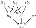
According to ω6, the paper resulting from the agents' collaboration will be accepted if and only if either it is submitted to the workshop and is readable or it is submitted to the conference and is of high quality. The state S′0 = (C ′0 , V ′ 0 ) such that C0 = {ω1, ω2, ω6} and V0 = {lt1, re, ac} is an equational state whose causal graph for the 3-agent case (n = 3) is illustrated in Figure 1. Note that the causal graph is acyclic, it is a DAG.
3 Conceptual Analysis
This section is devoted to discussing some concepts that play an important role in explanation. All concepts we consider can be seen as binary predicates whose first argument is the explanans (or the causing fact) and second argument is the explanandum (or the caused fact). We assume the explanans is always a term, namely, a non-empty conjunction of literals in which a propositional variable can occur at most once, while the explanandum can be any formula. We note Term the set of terms and λ, λ′ , . . . its elements. Given a non-empty Z ⊆ P, we note TermZ the set of terms built from the variables in Z. Given λ, λ′ ∈ Term, with a bit of abuse of notation, we write λ′ ⊆ λ (resp. λ′ ⊂ λ) to mean that the set of literals appearing in λ′ is a subset (resp. strict subset) of the set of literals appearing in λ.
3.1 Abductive Explanation
Following [Ignatiev et al., 2019], we define abductive explanation (AXp) from the concept of prime implicant. The term λ is said to be a prime implicant of φ (i.e., PImp(λ, φ)) if, necessarily λ entails φ and there is no λ′ ⊂ λ such that λ′ entails φ. Moreover, λ is said to be an abductive explanation of φ (i.e., AXp(λ, φ)) if it is a prime implicant of φ and is actually true. Both concepts are definable using the S5-modality □. 3 Let λ ̸= φ, then
Furthermore,
Let us continue Example 3 to illustrate the concept of abductive explanation.
Example 5 (cont.). Let the model (S0, SΓ0 ) be defined as in Examples 1 and 3. We have:
This means that at model (S0, SΓ0 ) the fact the first agent invests a large amount of time in the collaboration and the paper is submitted to the workshop abductively explains the fact that the paper is accepted.
The following proposition provides a dynamic characterization of prime implicant and abductive explanation, when the explanandum is a propositional formula and the model contains all states.
Proposition 1. Let λ ∈ Term, ω ∈ LPROP and (S, S) ∈ M. Then,
where, for every λ ∈ Term,
3 See also [Liu and Lorini, 2023] for a formal analysis of abductive, contrastive and counterfactual explanation of classifier systems based on the modal logic S5.
3.2 Causal Necessity Post Intervention
In this section, we define a new modality capturing causal necessity after intervention. We see an atomic intervention on a variable p as an event of type p = ⊤ or p = ⊥. A complex intervention is a finite set of atomic interventions with at most one atomic intervention for each variable. We define the set of complex interventions as follows:
Elements of Int are noted E,E′ , . . . Given {p1 = τ1, . . . , pk = τk} ∈ Int , we define its corresponding set of equational formulas
as well as its corresponding conjunction over variables:
For every finite set of atomic propositions Z ⊆ P, we note IntZ the set of interventions for Z, that is,
At the semantic level, a local intervention p = τ replaces any equational formula for p in a causal base by the equational formula p ↔ τ .
We can now define a modal operator of causal necessity post intervention E parameterized by a set of propositional formulas X:
with
[E,X]φ has to be read "φ necessarily holds after the intervention E relative to the causal base X". Notice π{p1=τ1,...,pk=τk},X is the operation that replaces all equational formulas for the variables p1, . . . , pk in the causal base X by the new equational formulas p1 ↔ τ1, . . . , pk ↔ τk.
In the next section, we will use the operator [E,X] to define the notion of actual cause.
3.3 Actual Cause
In this section, we deal with the concept of actual cause based on Halpern & Pearl's definition [Halpern and Pearl, 2001; Halpern and Pearl, 2005a]. We rely on the most recent formulation of this concept given in [Halpern, 2015]. We are going to show that the problem of checking whether a fact λ is the actual cause of another fact φ can be formulated as a model checking problem relative to an equational state.
Following Halpern, we say that λ is the actual cause of φ if i) both λ and φ are true, ii) it is possible to intervene on the endogenous variables in λ, while fixing by intervention the values of some endogenous variables that are not in λ, such that if the value of the exogenous variables do not change φ will be necessarily false, and iii) there is no λ′ ⊂ λ for which ii) holds. This notion of actual cause is only definable relative to equational states since it requires to distinguish exogenous from endogenous variables.
Definition 11 (Actual cause). Let S = (C, V ) ∈ SEq , U ⊆ S and λ ∈ Termend(S). We say λ is an actual cause of φ at (S,U) if the following holds:
where
and
Note that, in line with Halpern, we assume that the cause λ is built from the endogenous variables.
The conjunct λ ∧ φ ∧ But(S, λ, φ) in the definition captures the notion of sufficient cause. Together with the conjunct ∧λ′⊂λ ¬But(S, λ′ , φ) it makes actual cause to coincide with minimal sufficient cause.
The following example is a classic in the literature on formal models of causality. We use it to illustrate the previous definition.
Example 6. Suzy and Billy throw rocks at a bottle. There is an asymmetry between them. Suzy is stronger than Billy so that, if she throws her rock, her rock will get at the bottle first, shattering it and preventing Billy from hitting it with his rock. This means that i) Suzy throws her rock (st) iff she decides to do so (sd), ii) Billy throws his rock (bt) iff he decides to do so (bd), iii) Suzy hits the bottle (sh) if and only if she throws her rock (st), iv) Billy hits the bottle (bh) if and only if he throws his rock (bt) while Suzy does not hit the bottle (¬sh), v) the bottle is shattered (bs) if and only if either Billy or Suzy hits it. Thus, the causal base can be described as follows:
We suppose we are in the situation in which both Billy and Suzy decide to throw their rocks:
We define S0 = (C0, V0).
We suppose the universe U0 includes all states whose causal bases are closed under C0 and all possible rules that can be added to the causal base through an intervention on the variables of the problem. That is, we consider the universe SΓ0 with
We have that:
- st is an actual cause of bs at (S0, SΓ0 ),
- bt is not an actual cause of bs at (S0, SΓ0 ).
In his analysis of actual cause, Halpern restricts to acyclic causal models, namely, causal models in which dependency relations between variables contain no cycles. Following Halpern, we consider equational states whose induced causal graphs are DAGs. As the following proposition highlights, in such states once the values of the exogenous variables and of the irrelevant variables are fixed, there is a unique solution after an intervention.
Proposition 2. Let S = (C, V ) be an equational state such that its causal graph GS is a DAG and let E ∈ IntZ for some Z ⊆ end(S). Then, there is a unique S′ = (C ′ , V ′ ) such that
and
We denote with SE such a unique state.
Proposition 2 turns out to be crucial for proving the following theorem.
Theorem 12. Let S = (C, V ) be an equational state such that its causal graph GS is a DAG, λ ∈ Termend(S) and P(ω) ⊆ P(S). We have (S, S) |= But(S, λ, ω) iff
Theorem 12 highlights that in the case of acyclic causal structures the construction But(S, λ, ω) correctly captures the "but-for" clause, the core part of Halpern's definition of actual cause. In particular, according to Theorem 12, it is possible to intervene on the endogenous variables in λ, while fixing by intervention the values of some endogenous variables that are not in λ, such that the unique state resulting from these interventions in the which the values of the exogenous variables have not changed makes φ false.
4 Model Checking
In this section, we define model checking over finite Γmodels (Definition 6).
Definition 13 (Model checking).
input: a finite vocabulary Γ, a finite state S0 ∈ SΓ, and a formula φ0 ∈ L.
To be able to provide an efficient algorithm, we use a translation to Quantified Boolean Formulas (QBF).
Let Γ and φ0 be given. The set W of relevant sub-formulas is defined as follows: W = P(φ0) ∪ P(Γ) ∪ {△ω | ω ∈ Γ}.
A set of fresh propositional variables is defined for each state. That is, for each S ∈ SΓ, we have WS = {xφ,S | φ ∈ W}, where xφ,S is a fresh propositional variable not appearing in Γ or φ0.
Given an operation π, the sets of its expansions exp(π) and its retractions ret(π) are defined recursively, as follows.
It should be clear that operation π is equivalent to +exp(π)-ret(π), in the sense that SRπS′ iff SR+ exp(π)- ret(π)S′ .
The translation of the model checking problem (S, U) |= φ to QBF is recursively defined as follows.
Definition 14 (Translation).
Intuitively, each fresh variable xp,S encodes the membership of p to V , whereas x△α,S encodes the membership of α to C. This means that each state S ∈ SΓ can be associated with an element of 2WS , namely {xp,S | p ∈ V } ∪ {x△α,S | α ∈ C}. Therefore, we also have that formula Rπ (S,S′ ) encodes the membership of (S, S′ ) to the relation Rπ, as follows. If α is removed from the base of S, then △α is set to false in S′ . Similarly, if α is added to the base of S, then △α is set to be true in S′ . In the latter case, one must also make sure that S′ is a state. Therefore, tr(α, S′ ) is also set to be true at S′ . In the third case, if α is not added nor removed, then its truth value must remain the same in S′ . In addition, in the case where it is true, α must also be satisfied by S′ . Also note that the formulas △ω which are not in W are considered to be false in the model. Therefore, the translation replaces them with ⊥. The theorem below shows how the translation is used to encode model checking.
Theorem 15. Let S = (C, V ) be a state in SΓ. (S, SΓ) |= φ if and only if |=QBF ∀WS(DS → tr(φ, S)), where:
The following corollary is a direct consequence of Theorem 15 and the fact that the translation tr is polynomial.
| #agents | 3 | 16 | 64 | 256 |
|---|---|---|---|---|
| |P| | 7 | 20 | 68 | 260 |
| |W| = |P| + |Γ0| | 12 | 25 | 73 | 265 |
| |SΓ| = 2|W| | 4096 | 3.36e7 | 9.44e21 | 9.93e79 |
| Exec. time (sec.) | 0.0866 | 0.0891 | 0.1698 | 5.3242 |
Corollary 16. Model checking (Def. 13) is in PSPACE.
Note that, if the modal depth of φ is 1, we have only two quantifiers on the formula of Theo. 15. Therefore, in this case, model checking is in ΣP2 . This is the case of most examples of causality found in the literature, including examples 1-5 and 6.
In order to verify the feasibility of the theoretical framework, we implemented a symbolic model checker, 4 which uses the translation into QBF. The resulting QBF is then translated into a binary decision diagram (BDD), similar to what is done in [van Benthem et al., 2018]. The program is implemented in Haskell and the BDD library used is HasCacBDD [Gattinger, 2023]. It was compiled with GHC 9.4.8 in a MacBook Air with a 1.6 GHz Dual-Core Intel Core i5 processor and 16 GB of RAM, running macOS Sonoma 14.1.2.
Table 1 shows the performance of the symbolic model checker on different instances of Example 5. Execution times correspond to the elapsed time to perform (1). The number of states (|SΓ|) gives an idea of the size of the search space for formulas. In principle, to check a formula of the form □φ, one must check φ in every state of the model. Because of that, a naive implementation cannot be used.
5 Conclusion
We have presented a novel logical framework for causal reasoning in which causal information is represented through propositional causal bases. At the language level, its main constituent is a modality of causal necessity conditional on the occurrence of a causal change operation. We have used our language to express the notion of abductive explanation, representative of the PI-family, and of actual cause, representative of the CI-family. We have provided a PSPACE model checking procedure based on a polysize reduction to QBF and shown how to exploit it to automatically verify properties of explanations and causes. Our conjecture is that the model checking problem defined in Section 4 is PSPACE-hard. This, in conjunction with Corollary 16, would allow us to conclude that it is PSPACE-complete. We believe PSPACE-hardness is provable using a polysize reduction of the model checking problem for the modal logic K interpreted using belief bases. The latter problem was proved to be in PSPACE in [Lorini, 2019]. Future work will be devoted to proving this conjecture. We also plan to extend our analysis to the notion of NESS cause from the CI-family [Beckers, 2021b] and the notion of agency analyzed in STIT theory [Belnap et al., 2001].
4 Available: https://src.koda.cnrs.fr/tiago.de.lima/cmc/-/releases/ 0.1.0.0
Acknowledgments
Support from the ANR project ALoRS "Action, Logical Reasoning and Spiking networks" (grant number ANR-21-CE230018-01) and from the ANR AI Chair project "Responsible AI" (grant number ANR-19-CHIA-0008) is gratefully acknowledged.
@inproceedings{ijcai2024p368,
  title     = {Model Checking Causality},
  author    = {de Lima, Tiago and Lorini, Emiliano},
  booktitle = {Proceedings of the Thirty-Third International Joint Conference on
               Artificial Intelligence, {IJCAI-24}},
  publisher = {International Joint Conferences on Artificial Intelligence Organization},
  editor    = {Kate Larson},
  pages     = {3324--3332},
  year      = {2024},
  month     = {8},
  note      = {Main Track},
  doi       = {10.24963/ijcai.2024/368},
  url       = {https://doi.org/10.24963/ijcai.2024/368},
}
TY - CPAPER TI - Model Checking Causality AU - de Lima, Tiago AU - Lorini, Emiliano T2 - Proceedings of the Thirty-Third International Joint Conference on Artificial Intelligence, IJCAI-24 PB - International Joint Conferences on Artificial Intelligence Organization PY - 2024 SP - 3324 EP - 3332 DO - 10.24963/ijcai.2024/368 UR - https://doi.org/10.24963/ijcai.2024/368 ER -Copied
Machine-readable versions of this paper, for tools and AI agents:





