A Rule-Based Modal View of Causal Reasoning

1 Introduction

Causal reasoning is a central topic for AI nowadays given the importance of causal concepts such as (causal) explanation and responsibility for AI applications. It is an area of research at the crossroad of different disciplines ranging from logic and philosophy to economics.

Two approaches to the formalization of causal reasoning should be distinguished. On the one hand, we have the rule-based (or syntactic) approach whereby causal laws are seen as rules expressed in a given logical language, such as propositional logic. This approach grounds on and is tightly interconnected with earlier work on non-monotonic reasoning in the area of knowledge representation [Geffner, 1990; Lifschitz, 1997; McCain and Turner, 1997; Bochman, 2003; Giunchiglia et al., 2004]. The recent work by Bochman, culminated in [Bochman, 2021], is representative of this approach. It relates the rule-based approach to the theory of counterfactuals [Bochman, 2018b] and actual causality [Bochman, 2018a].

On the other hand, we have the structural equation modeling (SEM) approach whereby the causal connections between variables are expressed via a system of structural equations. Pearl's work on causality [Pearl, 2009] is probably the most famous example. The SEM approach has been successfully applied to formalizing a wide variety of concepts relevant to AI including actual causality [Halpern, 2008; Halpern, 2016; Beckers and Vennekens, 2017; Beckers, 2021], explanation

[Woodward, 2003; Woodward and Hitchcock, 2003; Halpern and Pearl, 2005b], responsibility and blame [Chockler and Halpern, 2004; Alechina et al., 2017; Halpern and KleimanWeiner, 2018], discrimination [Chockler and Halpern, 2022]. The relationship between the rule-based and the SEM approach was explored in [Bochman and Lifschitz, 2015], where it was shown that structural equation models are representable in the causal calculus introduced in [Bochman, 2003; Giunchiglia et al., 2004]. In the general SEM setting, for every endogenous variable and for every value assignment for the other variables (endogenous and exogenous ones), we must specify the value that the variable will take.

In the present work, we introduce a novel rule-based semantics for a number of modal languages that support reasoning about causality. It relies on the notion of causal base, i.e., a set of explicit causal information in propositional form. Our proposal is related to some recent work in the area of epistemic logic devoted to comparing the extensional semantics of epistemic logic based on Kripke models with a succinct semantics using belief bases [Lorini, 2018; Lorini, 2019; Lorini, 2020]. Here we make an analogous operation: we compare the SEM semantics for modal languages of causality with a succinct semantics using causal bases.

The general purpose of this paper is twofold. First of all, we want to show that, when variables are assumed to be Boolean, causal reasoning can be performed via classical deductive reasoning within a standard modal framework in which causal information is expressed in propositional form. We firmly believe that Boolean (or binary) causal models are interesting per se since they cover, or at least are closely connected with, a variety of interesting models and concepts including propositional opinion diffusion [Grandi et al., 2015; Christoff and Grossi, 2017], binary neural networks and diagrams [Lewis, 1986; Hubara et al., 2016; Narodytska et al., 2018; Shi et al., 2020], Boolean networks [Kauffman, 1969]. Secondly, we want to shed light on the intimate connection between causal reasoning and epistemic reasoning that, we believe, is difficult to grasp using the SEM approach. Our rule-based semantics, which leverages the concept of causal base analogous to that of belief base, makes this task easier.

Outline. The paper is organized as follows. In Section 2, we discuss related work in more detail. In Section 3, we introduce our rule-based semantics as well as a modal language for reasoning about the notions of causal necessity and possibility interpreted over it. We provide complexity results for both satisfiability and model checking for this language. Section 4 is devoted to exploring the relationship between our rule-based semantics and the SEM semantics. We show that the latter corresponds to a specific instance of the former where causal information is represented in an equational form. In Section 5, we extend the basic framework by interventionist conditional operators in Halpern & Pearl's style [Halpern, 2000; Halpern and Pearl, 2005a]. We introduce a novel semantics for interventionist conditionals relying on the concept of replacement and again compare it with the SEM semantics. Our semantics helps to better understand the relationship between intervention and belief change. Intervention is seen as a replacement operation, a kind of operation originally introduced in the theory of belief change to replace one sentence by another in a belief base [Hansson, 2009]. Finally, in Section 6, we present a second extension with Lewisian conditional modalities [Lewis, 1973]. We interpret them by means of a notion of comparative similarity that we compute from the causal base. We compare the Lewisian conditional modality with the interventionist modality and spell the conditions under which the latter can be seen as a special case of the former. Moreover, we elucidate the relationship between our rule-based semantics for counterfactual conditionals and the update semantics of belief base contraction and revision.

2 RelatedWork

Structural equation models have been exploited as a semantics for a number of modal languages of interventionist conditionals [Galles and Pearl, 1998; Halpern, 2000; Halpern and Pearl, 2005a]. Both the axiomatic and the complexity aspects of these modal languages have been investigated [Galles and Pearl, 1998; Halpern, 2000] as well as their connection with the logic of counterfactual conditionals [Halpern, 2013; Zhang, 2013]. The SEM semantics used in these works is more general than our ruled-based semantics, since variables are not necessarily Boolean. However, it has the disadvantage of not being succinct, thereby making model checking for these modal languages of causality not exploitable in practice. Models used there are huge: every endogenous variable is associated to a function that fully describes how the value of the variable varies depending on the values of the other (endogenous and exogenous) variables. This description of the causal system is exponential in the number of variables. For instance, in the Boolean case, if there are n endogenous variables and m exogenous ones, a table with n × 2(n+m)-1 entries (i.e., 2(n+m)-1 entries for each endogenous variable) is needed. Moreover, the description of the causal system becomes infinite if there is an infinite number of variables. Our rule-based semantics does not have this limitation. As we will shown in Section 4, we can fully describe a causal system with a set of equational formulas of polynomial size, even in the infinite variable case. This is appealing from the point of view of formal verification.

It is also important to underline some differences between our approach to causal reasoning and Bochman's approach cited above. Ours is a classic work in modal logic. At the syntactic level, we start with a basic modal language for reasoning about causal necessity. We borrow from [Burks, 1951] the idea of modeling causal necessity by means of a normal modality S5. Then, we extend it with dyadic modal operators for interventionist and Lewisian conditional. At the semantic level, we use accessibility relations over possible states/worlds for interpreting the different modal operators. Bochman's language presented in [Bochman, 2018b] is not a modal language in the usual modal logic sense. Namely, it is not an extension of the propositional language with different modal operators, in which we can write any Boolean combination of propositional formulas and modal formulas as well as formulas with nested modalities. His semantics does not use accessibility relations over possible worlds/states. His language consists of causal rules of the form A ⇒ B, where A and B are propositional formulas. He uses a nonmonotonic semantics based on the notion of exact model for a set of causal rules, that is, a consistent set of information that is closed under the causal rules and in which every information is explained by other information in the set. Given the significant differences between the two approaches, we do not know whether and how our concept of causal necessity, and the satisfiability and model checking problem defined in our framework can be "translated" into his framework.

3 Logical Framework

In this section, we introduce a simple modal language for reasoning about causality. Following [Lorini, 2020], the semantics of our language uses the notion of "state" consisting of (i) a causal base, including all causal information which regulates the physical world, and (ii) a valuation of propositional facts that is compatible with the causal information. At the syntactic level, our language extends propositional logic by an operator for representing explicit causal information and another operator for representing causal necessity of facts.

3.1 Semantics

Assume a countably infinite set of atomic propositions P = {p, q, . . .} and let LPROP(P) be the propositional language built from P. We assume the language LPROP(P) contains the symbol ⊤ ("true") as primitive, while ⊥ ("false") is defined from it as usual ⊥ =def ¬⊤.

Given a propositional formula ω ∈ LPROP(P), the set of symbols from P occurring in ω is noted P(ω). The definition extends to a set of propositional formulas X ⊆ LPROP(P) in a straightforward manner: P(X) = ⋃ω∈X P(ω). The main constituent of our semantics is the following notion of state.

Definition 1 (State). A state is a pair S = (C, V ) where C ⊆ LPROP(P) is a causal base and V ⊆ P is a propositional valuation such that

with V |= ω meaning that the propositional formula ω is true under the valuation V and defined inductively, as usual.

The set of all states is noted S. A state S = (C, V ) is said to be finite if both C and V are finite. The set of finite states is noted SFin .

The valuation V represents the actual environment and is assumed to be compatible with the information of the actual causal base. That is, if ω is included in the actual causal base (i.e., ω ∈ C) then it should be true in the actual environment (i.e., V |= ω).

We use the generic term "causal information" to indicate propositional formulas in a causal base. We use the more specific term "causal rule/law" for information in a causal base expressed through single implication ω1 → ω2 or double implication ω1 ↔ ω2. With a slight abuse of terminology, we call our semantics a rule-based semantics. To be more precise, it should be called a semantics based on causal information in propositional form. We stick to the former naming since it is more concise. The following definition introduces the notion of causal compatibility.

Definition 2 (Causal compatibility). We define ≡c to be the binary relation on the set S such that, for every S = (C, V ), S′ = (C ′ , V ′ ) ∈ S:

S ≡c S′ means that state S and state S′ are causally compatible since they share the same causal information. It is easy to verify that ≡c is an equivalence relation and that the following holds for every S = (C, V ), S′ = (C ′ , V ′ ) ∈ S:

The latter means that the causal information of the actual state must be true at all states that are causally compatible with it. To see this, suppose S ≡c S′ . Thus, by Definition 2, C ⊆ C ′ . Moreover, by definition of S, ∀ω ∈ C ′ , we have V ′ |= ω. Hence, since C ⊆ C ′ , ∀ω ∈ C, V ′ |= ω.

3.2 Language

In this section, we define a two-layer modal language for talking about explicit causal information and causal necessity. It is defined by the following grammar:

where p ranges over P and ω ranges over LPROP(P). The other Boolean connectives ∨,→ and ↔ are defined in the usual way. The first layer language LCI(P) (Language for Causal Information) is the language for talking about explicit causal information. The formula △ω has to be read "the information ω is causally relevant" or "information α is part of the causal description of the actual state". The second layer language LCIN(P) (Language for Causal Information and Necessity) extends the first layer by a modal operator □ for causal necessity in Burks' style [Burks, 1951]. In particular the formula □ϕ has to be read "it is causally necessary that ϕ" or, by adopting Burks' reading, "ϕ is true on causal grounds". As usual, we define ♦ϕ =def ¬□¬ϕ, where the formula ♦ϕ has to be read "it is causally possible that ϕ".

The language LCN(P) (Language for Causal Necessity) is the fragment of LCIN(P) in which we can only talk about causal necessity:

where p ranges over P. LPCN(P) (Language for Propositional Causal Necessity) is the fragment of LCN(P) in which we can only talk about the causal necessity of propositional facts. It is defined by the following grammar:

where p ranges over P and ω ranges over LPROP(P).

To sum up, we consider four languages LCI(P), LCIN(P), LCN(P) and LPCN(P) with the following inclusion relations:

LCIN(P) is the most general one. We interpret its formulas relative to a set of states U and a specific state S included in it. We call U context (or universe) of interpretation. (We omit semantic interpretations for the Boolean connectives ¬, ∧ and for ⊤ since they are defined in the usual way.)

Definition 3 (Semantic interpretation). Let U ⊆ S and S = (C,V) ∈ U. Then:

The causal necessity modality □ is a so-called S5 modality. According to the previous definition, it is causally necessary that ϕ iff, ϕ is true at all states in the context that are causally compatible with the actual state. The modality △ has a settheoretic interpretation: the information ω is causally relevant if it is included in the actual causal base. For notational convenience, we write S |= ϕ instead of (S, S) |= ϕ. S is also called the global context.

As highlighted by the following proposition, the causal necessity of a propositional fact coincides with its deducibility from a causal base.

Proposition 1. Let S = (C,V) ∈ S and ω ∈ LPROP(P). Then, S |= □ω iff ω ∈ Cn(C), with Cn the classical deductive closure operator over the propositional language LPROP(P).

As a simple example to illustrate the semantics, consider the state S = ({ω1, ω2}, ∅) with ω1 = (p1 ∧ ¬p2) → p3 and ω2 = p4 → ¬p2. We have that the causal information ω1 and ω2 are relevant at state S and this is a causal necessity, that is, S |= (△ω1 ∧△ω2) ∧□(△ω1 ∧△ω2 ). Furthermore, it is causally necessary that "if p1 and p4 then p3", that is, S |= □((p1 ∧ p4) → p3 ).

3.3 Satisfiability andModel Checking

A formula ϕ ∈ LCIN(P) is said to be satisfiable if there exists a context U ⊆ S and a state S ∈ U such that (S, U ) |= ϕ.

Satisfiability checking problem

Given: ϕ ∈ LCIN(P).

Question: Is ϕ satisfiable?

We formulate model checking as the problem of verifying whether a formula is true at a given finite state.

Model checking problem

Given: ϕ ∈ LCIN(P) and S ∈ SFin .

Question: Do we have S |= ϕ?

The first result of this section highlights that satisfiability checking for the language LCIN(P) as well as for its fragments LCN(P) and LPCN(P) has the same complexity as SAT. The proof of the theorem relies on the fact that for any satisfiable formula we can construct a model of polynomial size which satisfies it.

Theorem 1. Let Λ ∈ {CIN, CN, PCN}. Then, satisfiability checking for LΛ(P)-formulas is NP-complete.

In our framework model checking has the same complexity as satisfiability checking. This is due to its compact formulation which makes it different from standard model checking for the modal logic S5 over Kripke models which is known to be polynomial with respect to the size of the input formula to be checked and the size of the input model [Gr¨adel and Otto, 1999].

In order to prove NP-hardness of model checking, we use a a polynomial reduction of SAT to it. In order to prove its NP-membership, we rely on the construction that we use for proving Theorem 1.

Theorem 2. Let Λ ∈ {CIN, CN, PCN}. Then, model checking for LΛ-formulas is NP-complete.

4 Relation with Structural EquationModels

In this section we study the connection between our rulebased semantics for causal reasoning and the SEM semantics. We first define a subclass of states in the sense of Definition 1, called equational states, in which an information in a causal base can only be expressed in equational form: a rule specifying the necessary and sufficient condition for making a certain atomic proposition true. Then, we define a variant of structural equation models in which variables are assumed to be binary (viz. Boolean). We call them binary causal models (BCMs). We show that BCMs are essentially equivalent to equational states as far as reasoning about propositional causal necessity is concerned.

4.1 Equational States

Let LEQ(P) be the the fragment of the propositional language LPROP(P) which contains equational formulas:

An equational state is finite state whose causal information is expressed in equational form and which includes at most one equational formula for each variable.

Definition 4 (Equational state). A state S = (C, V ) is said to be in equational form if and only if C is finite, C ⊆ LEQ(P), V ⊆ P(C) and

The set of states in equational form, or equational states, is noted SEq .

As a side note, model checking for equational states is also NP-complete. NP-membership is evident because of Theorem 2. The proof of NP-hardness uses the same argument as the proof of NP-hardness for Theorem 2: polynomial reduction of SAT to model checking.

An interesting aspect of equational states is their graphical counterpart. Specifically, given an equational state S = (C,V), we can extract the causal graph ΓS = (NS,PS ) with NS = P(C) and where the causal parent function PS : N -→ 2N is defined as follows, for every p ∈ N :

where P+(ω) = P(ω) ∪ {⊤} if ⊤ occurs in ω, and P+(ω) = P(ω) if ⊤ does not occur in ω. In equational states we can partition the set of variables into two sets: the set of exogenous variables and the set of endogenous ones. Specifically, a variable p is said to be exogenous in state S if it has no parents in the corresponding causal graph ΓS (i.e., PS(p) = ∅), it is said to be endogenous in S otherwise. As the following proposition highlights, an endogenous variable behaves functionally, i.e., its truth value is entirely determined by the truth values of the other variables.

Let us focus on an example of social influence in a multiagent setting in order to illustrate the concept of equational state and its graphical counterpart.

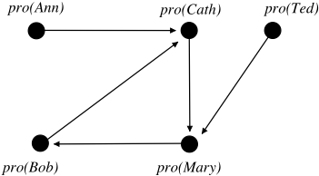
Example 1. Consider a set of five agents Agt = {Ann,Bob,Cath,Mary,Ted}. Each agent has an opinion about the use of nuclear energy for electricity production. In particular, she/he can be either in favor of or against it. An agent's opinion may be influenced by and depend on other agents' opinions. In order to represent agents' opinions, we suppose P includes atomic propositions of type pro(x) with x ∈ Agt , pro(x) meaning that x is favor and ¬pro(x) meaning that x is against the use of nuclear energy for electricity production. We assume we have perfect information about the dependency relations between the variables. In particular, we know that variables pro(Ann) and pro(Ted) are exogenous (i.e., Ann and Ted's opinions are independent of the other agents' opinions), while all other variables are exogenous. The causal connections between the variables are described by the following three equational formulas:

The three formulas express, respectively, that (i) Cath will be in favor of the use of nuclear energy if and only if Ann and Bob are unanimously in favor (ω1), (ii) Mary will be in favor if and only if Ted is in favor in case Cath is in favor too (ω2), and (iii) Bob is in favor if and only if Mary is in favor (ω3). Consider the state S = ({ω1, ω2, ω3}, {pro(x) : x ∈ Agt}). It is straightforward to verify that S is an equational state. The (influence) causal graph induced by it is represented in Figure 1. Clearly, there exists at least one state which is compatible with the causal information ω1, ω2, ω3:

Moreover, at state S it is causally necessary that Bob is in favor of the use of nuclear energy. In other words, Bob has no freedom, he is trapped in the influence process:

Moreover, it is not causally possible that Cath is in favor while Ted is against:

As the following theorem indicates, for every formula of the language of causal necessity, there exists a mapping from finite states to equational states such that the input state satisfies the formula if and only if the output state satisfies it too.

Theorem 3. Let ϕ ∈ LCN(P). Then, there exists a function g : SFin -→SEq such that

From Theorem 3 we can conclude that for every formula of the language of causal necessity to be checked relative to a finite state, we can transform the latter into an equational state and check the formula relative to it. In other words, the general model checking problem defined in Section 3.3 can be reduced to model checking relative to equational states.

The theorem relies on the fact that, given a formula ϕ, we can transform a finite causal base C into a causal base C ′ containing a single equational formula ωeq such that the set of propositional interpretations for the atoms in P(ϕ) satisfying all formulas in C is the same as the set of propositional interpretations for the atoms in P(ϕ) satisfying ωeq. This guarantees that from a finite state S = (C, V ) we can build an equational state S′ = ({ωeq},V ′ ) such that S |= ϕ iff S′ |= ϕ. However, the transformation is exponential. The equational formula ωeq uses the canonical DNF of the Boolean function representing the set of interpretations for the atoms in P(C) that satisfy all formulas in C. The size of a such a canonical DNF is exponential in the size of P(C). We believe it is not possible to find a polynomial transformation of a finite state into an equational state that guarantees equisatisfaction of ϕ.

Note that Theorem 3 cannot be generalized to the more general language LCIN(P) since states in SEq only allow causal information to be expressed in an equational form.

4.2 Binary Causal Model

Before defining the notion of binary causal model some preliminary notions are needed. A binary assignment for the set of variables X ⊆ P is a function

The set of binary assignments for X is noted AsgX. Interpretation |.| of propositional formulas in LPROP(X) relative to assignments in AsgX is as usual: |p|Asg X = {IX ∈ AsgX : IX(p) = 1} for p ∈ X; |⊤|Asg X = AsgX; |¬ω|Asg X = AsgX \ |ω|Asg X ; |ω ∧ ω′ |Asg X = |ω|Asg X ∩ |ω′ |Asg X .

Definition 5 (Binary causal model). A binary causal model (BCM) is a tuple Θ = (Vexo , Vend , (Fp)p∈Vend ) where Vexo is a finite set of exogenous variables, Vend is a finite set of endogenous variables such that Vend , Vexo ⊆ P and Vend ∩ Vexo = ∅, and, for every p ∈ Vend :

For notational convenience, we sometimes abbreviate V \ {p} as p. Moreover, when the context is unambigous, we write Asg instead of AsgV and note I, I ′ , . . . its elements.

Definition 6 (Solutions of a BCM). Let Θ = (Vexo , Vend , (Fp)p∈Vend ) be a BCM and let I ∈ Asg . We say that I is a solution of Θ if and only if, for every p ∈ Vend :

where I|p is the restriction of function I to p. The set of solutions of Θ is noted Sol (Θ).

Definition 7 (Pointed BCM). A pointed BCM is a pair (Θ, I) with Θ = (Vexo , Vend , (Fp)p∈Vend ) a BCM and I ∈ Sol (Θ). The class of pointed BCMs is noted B.

Pointed BCMs provide a natural semantics for interpreting formulas of the language of propositional causal necessity. In particular, given a pointed BCM (Θ, I) with Θ = (Vexo , Vend , (Fp)p∈Vend ) we can interpret formulas of the language LPCN(V), as follows. (Boolean cases and ⊤ are again omitted since they are defined in the standard way.)

Notice in particular the interpretation of the causal necessity modality □: it is causally necessary that ω if ω is true for all solutions of the actual causal model.

The following theorem highlights the tight similarity between equational states and pointed BCMs. Every equational state can be mapped into a pointed BCM and, conversely, every pointed BCM can be mapped into an equational state such that the truth of the formulas in the language of propositional causal necessity is invariant between them.

Theorem 4. There exists a surjection f : SEq -→ B such that if f(S) = (Θ, I) with Θ = (Vexo,Vend, (Fp)p∈Vend ) then

Note that Theorem 4 is conceptually stronger than Theorem 3 since the function f works for all formulas in the language LPCN(V), while the function g in Theorem 3 only works for a single formula in the language LCN(P).

5 Interventionist Conditionals

In this section, we are going to define a semantics for interventions which relies on a replacement operation on causal bases in Hansson's style [Hansson, 2009]. We will show that, when restricting to equational states, it corresponds to the SEM semantics for interventions [Halpern, 2000; Halpern and Pearl, 2005a]. Before introducing the semantics, we first define the syntax of interventionist conditional modalities.

5.1 Syntax

The antecedent of an interventionist conditional is an event, namely, a set of basic interventions on propositional variables of the form p=1 (the variable p is set to 'true') or p=0 (the variable p is set to 'false') with at most one intervention per variable. The set of basic interventions is defined as follows:

while the set of events is defined as follows:

Elements of Evt are noted E, E ′ , . . . For notational convenience, given p=τ ∈ Int, we define its corresponding equational formula as follows: eq(p=1) = p ↔ ⊤ and eq(p=0) = p ↔ ⊥. We extend function eq to sets in the expected way: eq ({p1=τ1, . . . , pk=τk}) = {eq(p1=τ1), . . . , eq(pk=τk)}. Moreover, for each E ∈ Evt, we define the partial function valE with domain P and codomain {0, 1}: valE(p) = 1 if p=1 ∈ E, valE(p) = 0 if p=0 ∈ E, and undefined otherwise.

We consider the following extension of the language LPCN(P) by interventionist conditional operators of the form [E] and their negation:

LPCN-Int(P) with ϕ ranging over LPCN(P), ω ranging over LPROP(P) and E ∈ Evt. LPCN-Int stands for "Language for Propositional Causal Necessity plus Interventions". The new formula [E]ω has to be read "it will be causally necessary that ω, after the occurrence of the event E" or "if the event E occurred, ω would be necessarily true". As usual, we define 〈E〉ω =def ¬[E]¬ω. Note we only allow negation over arbitrary formulas in LPCN(P) and over the modality [E]. Indeed, we are merely interested in talking about causal necessity (i.e., [E]) and causal possibility (i.e., 〈E〉) of propositional facts after intervention. Negation over arbitrary formulas in LPCN-Int(P) (i.e., ¬γ) would add unnecessary complications that we prefer to leave aside for the moment.

Note also we could have built the extension with interventionist conditionals on the top of the language LCIN(P) instead of the more restricted language LPCN(P). We did not do this since the language LPCN-Int(P) is sufficient to achieve our goal of comparing the interpretation of the concept of intervention in the rule-based semantics with its interpretation in the SEM semantics. The complexity upper bound for model checking we will provide in the next section generalizes straightforwardly to the more general language for interventionist conditionals built on the top of LCIN(P).

5.2 Semantics

In order to define interventionist conditionals semantically, some preliminary notions are needed. The effect of an event (a set of interventions) is to add information about the truth values of certain propositional variables to the causal base and to remove from the causal base all equational formulas about those variables. The latter is called the revocable part of the causal base in the light of the event. In other words, the revocable part of a causal base C in the light of an event E, noted Rev(C,E), includes all causal information that is superseded by some intervention in E.

Definition 8 (Revocable part of a causal base). Let C ⊆ LPROP(P) and E ∈ Evt . We define

The following definition introduces the notion of causal compatibility post intervention.

Definition 9 (Causal compatibility post intervention). Let E ∈ Evt . We define ⇒E to be the binary relation on the set of states S such that, for every S = (C, V ), S′ = (C ′ , V ′ ) ∈ S:

S ⇒E S′ means that state S′ = (C ′ ,V ′ ) is compatible with state S = (C,V) after the occurrence of event E. According to previous definition, the latter is the case if the causal base C ′ is the result of the following replacement operation applied to the causal base C: (i) remove from the causal base C all formulas which are revocable in the light of the event E, and then (ii) add to the resulting base the equational formulas corresponding to the interventions in E.

By means of the relation ⇒E , we can provide a semantic interpretation of the interventionist modalities [E]. They, too, are interpreted relative to a set of states (a context) and a specific state S included in it. Let U ⊆ S and S ∈ U . Then,

The other constructs of the language LPCN-Int(P) (i.e., ϕ, ¬[E]ω and γ ∧ γ) are interpreted in the usual way. Again, to simplify notation, we write S |= γ instead of (S, S) |= γ. Note that the interventionist modality with the empty event coincides with the causal necessity operator, i.e., the formula [∅]ω ↔ □ω is valid.

The following theorem provides a complexity upper bound of model checking for the language extended with interventionist modalities. Its proof relies on two facts: (i) the formula to be checked is a conjunction of the form γ1 ∧ . . . ∧γm where each conjunct is of the form ϕ, [E]ω or ¬[E]ω with ϕ ∈ LPCN(P), (ii) model checking the formula [E]ω relative to a finite state is reducible to model checking the formula □(∧p=τ∈E eq(p=τ) → ω) ∈ LPCN(P) relative to the finite state obtained from the input state through the removal of all causal information which is revocable in the light of the event E. Thus, thanks to Theorem 2, model checking for LPCN-Int(P)-formulas is solvable by a poly-time deterministic Turing machine querying an NP-oracle.

Theorem 5. Model checking for LPCN-Int(P)-formulas is in P NP =∆P2 .

Let us go back to our running example.

Example 2 (cont.). Let us consider again the equational state S = ({ω1, ω2, ω3}, {pro(x) : x ∈ Agt}) as defined in Example 1. We have shown that in this state Bob cannot be against the use of nuclear energy and that Cath cannot be in favor while Ted is against. It is interesting to observe that, by forcing Cath to be in favor of the use of nuclear energy through intervention on her opinion we cut the influence of Ann and Bob's opinions on her opinion. Consequently, (i) it becomes possible for Bob to be against the use of nuclear energy, and (ii) it becomes possible for Cath to be in favor while Ted is against. Formally, we have:

However, the intervention pro(Mary)=1 does not open the possibility for Bob to be against when Ted is in favor:

5.3 Back to Structural Equational Models

Before concluding, it is worthwhile to explore the connection between the rule-based semantics for interventionist conditionals defined in the previous section and the standard SEM semantics. The following definition specifies the way a BCM is updated through an event. Our definition is slightly different from the update semantics used in the SEM literature whereby interventions only apply to endogenous variables, and the partition of the set of variables into exogenous and endogenous ones does not change under intervention. We assume interventions can also apply to exogenous variables thereby transforming them into endogenous ones. The justification is that we take exogenous and endogenous variables as part of the BCM relative to which formulas are evaluated.

Definition 10 (BCM after intervention). Let Θ = (Vexo,Vend, (Fp)p∈Vend ) be a BCM and E = {p1=τ1, . . . , pk=τk} ∈ Evt. We define the BCM resulting from the update of Θ by E as the tuple ΘE = (VE exo , VE end , (F E p )p∈VE end ) such that

The condition Range(F E p ) = {valE(p)} just means that F E p (Ip) = valE(p) for every Ip ∈ Asgp.

The modality [E] has the following interpretation relative to a pointed BCM:

This means that the conditional expression [E]ω holds if the consequent ω is true for all solutions of the actual BCM updated by the event E.

The following theorem is a generalization of Theorem 4 to the language LPCN-Int(V): there exists a truth preserving onto relation between equational states and BCMs for the language extended by interventionist modalities.

Theorem 6. There exists a surjection f : SEq -→ B such that if f(S) = (Θ, I) with Θ = (Vexo,Vend, (Fp)p∈Vend ) then

6 Lewisian Conditionals

In this section, we introduce a notion of counterfactual conditional interpreted by means of a comparative similarity relation. In the standard analysis of counterfactual conditionals the notion of similarity is given as a primitive [Lewis, 1973] or replaced by an abstract selection function [Stalnaker, 1968] which selects for every world and formula ϕ the set of most similar ϕ-worlds to it. In line with Ginsberg's earlier work on the computationally grounded semantics for counterfactuals [Ginsberg, 1986], we compute the comparative similarity relation from causal bases.

6.1 Semantics

A straightforward way to compute the comparative similarity relation between states relative to a causal base is by comparing the causal information of the causal base that is relevant in each state. This idea is made precise by the following definition.

Definition 11 (Similarity relation between states). Let S = (C,V), S′ = (C ′ ,V ′ ), S′′ = (C ′′ ,V ′′ ) ∈ S. We say that state S′ is at least as similar to state S as state S′′ is, noted S′′ ⪯S S′ , if

According to the previous definition, state S′ is at least as similar to state S as state S′′ is, if the set of causal information shared by S and S′′ is included in the set of causal information shared by S and S′ . In other words, state S′ is at least as causally compatible with state S as state S′′ is. This criterion is qualitative since it relies on set inclusion. A quantitative criterion, which is not studied here, would be based on comparing the two cardinalities |(C ∩ C ′′ )| and |(C ∩ C ′ )|.

Following Lewis, we use the similarity relation to define the set of closest (or most similar) states to a given state satisfying a given property ϕ.

Definition 12 (Set of ϕ-closest states). Let U ⊆ S, S = (C, V ) ∈ U and ϕ ∈ LCIN(P). We define

Closest(ϕ,S,U) is the set of closest ϕ-states to S in U, according to the similarity relation ⪯S. For notational convenience, we write Closest (ϕ,S) instead of Closest (ϕ,S,S).

On the syntactic side, we extend the modal language LCIN(P) introduced in Section 3.2 by counterfactual conditional modalities in Lewis' style of the form ϕ1 �ϕ2, with

ϕ1, ϕ2 ∈ LCIN(P), and interpret them relative to a context U ⊆ S and a state S ∈ U :

According to the previous semantic interpretation, the conditional ϕ1 � ϕ2 (read "if ϕ1 were true, ϕ2 would be true") holds at a given state S relative to the context U in case ϕ2 is true at all the closest ϕ1-states to S in U .

6.2 Relationship with Belief Change

There is a tight correspondence between counterfactual conditionals whose antecedents and consequents are expressed by propositional formulas and causal base change operations. In order to elucidate this correspondence the notion of ωremainder, borrowed from formal models of theory change [Alchourr´on et al., 1985] and belief base change [Hansson, 1993], is needed.

Definition 13 (ω-remainder). Let C ⊆ LPROP(P), ω ∈ LPROP(P) and C ′ ⊆ C. We say that C ′ is a ω-remainder of C if

where we recall that Cn is the classical deductive closure operator over the propositional language LPROP(P). We note C⊥ω the set of all ω-remainders of C.

According to the previous definition, an ω-remainder of a causal base C is a maximal subset of the original causal base from which the propositional fact ω is not deducible. The following theorem is the first key result of this section. It highlights the strong connection between counterfactual conditionals and the notions of base contraction and revision.

Theorem 7. Let S = (C, V ) ∈ S and ω1, ω2 ∈ LPROP(P). Then, the following three items are equivalent:

According to the previous theorem, declaring that a counterfactual statement ω1 � ω2 with propositional antecendent ω1 and consequent ω2 be true at a certain state is the same as stating the causal necessity of the fact that the antecedent implies the consequent relative to every ω1remainder of the actual causal base. Moreover, by virtue of Proposition 1, the latter is equivalent to declaring that the consequent ω2 is included in the deductive closure of each ω1remainder of the actual causal base after expanding it by ω1. This operation is called full meet belief base revision scheme or simple base revision in the belief revision literature [Fagin et al., 1983; Ginsberg, 1986; Nebel, 1989; Nebel, 1991; del Val, 1992; Rott, 1993].

The equivalence between items 1 and 3 in Theorem 7 is in line with the so-called Ramsey test [Stalnaker, 1968]. According to the latter, the validity of an epistemic conditional can be verified by adding the antecedent to a stock of beliefs, revising it if necessary, and checking whether the consequent is deducible from the resulting epistemic state.

6.3 Relationship with Interventionist Conditionals

The second key result of this section relates interventionist conditionals to Lewisian conditionals. It pinpoints a condition under which an interventionist conditional can be reduced to a Lewisian conditional.

Theorem 8. Let S ∈ SEq . Then,

According to the previous theorem, when considering equational states, if after the intervention there exists at least one state which is compatible with the causal base, then declaring that "ω will be causally necessary after intervention" is the same as declaring that "if all information corresponding to the intervention holds, ω would be true". More generally, if we restrict to equational states - that as shown in Sections 4.2 and 5.3 correspond to BCMs - the existence of a solution after intervention guarantees the reducibility of the interventionist conditional to a Lewisian conditional.

7 Conclusion

We hope we have successfully shown that our rule-based semantics offers a natural framework (i) for modeling some crucial concepts in the theory of causality including causal necessity and possibility, interventionist and counterfactual conditional, and (ii) for elucidating the connection between causal reasoning and epistemic reasoning, with special emphasis on belief base change. We have mainly focused on the complexity of satisfiability and model checking.

Future work will be devoted to studying the proof-theoretic aspects of the different modal languages introduced in the paper. We also intend to explore the practical implications of our work. We have shown that reasoning in our framework is in NP when dealing with causal necessity and possibility and in P NP in the extension by interventionist conditionals. We plan to come up with reductions of our satisfiability and model checking problems to SAT with the aim of automating causal reasoning.

Last but not least, we plan to use our framework for formalizing some interesting causal concepts with special attention to actual causality and causal explanation. As recently shown in [Beckers, 2021], the SEM semantics can successfully formalize different notions of actual cause including the Halpern & Pearl's definition [Halpern and Pearl, 2005a], the famous NESS (Necessary Element of a Sufficient Set) definition [Wright, 1988] and a counterfactual variant of the NESS definition. The correspondence results between equational states and binary SEMs we proved (Theorems 4 and 6) guarantee that all these definitions can be formalized in our semantics as well, provided that the variables are binary. In order to model causal explanation, we will extend our modal languages for causal reasoning with epistemic operators. Indeed, we conceive an explanation as a causal attribution by an explainer, namely, as a belief of the explainer about the actual cause of a given fact or event.

Acknowledgments

Support from the ANR project ALoRS "Action, Logical Reasoning and Spiking networks" (grant number ANR-21-CE230018-01) and the ANR-3IA Artificial and Natural Intelligence Toulouse Institute (ANITI) is gratefully acknowledged.