
On the Computation of Example-Based Abductive Explanations for Random Forests
Proceedings of the Thirty-Third International Joint Conference on Artificial Intelligence. Main Track. Pages 3679-3687.
https://doi.org/10.24963/ijcai.2024/407
Keywords
- Knowledge Representation and Reasoning: KRR: Computational complexity of reasoning
- Constraint Satisfaction and Optimization: CSO: Applications
- Machine Learning: ML: Explainable/Interpretable machine learning
Abstract
We show how to define and compute example-based abductive explanations. Such explanations are guaranteed to be 100% correct, fairly general, and persuasive enough since they cover sufficiently many reference instances furnished by the explainee. We prove that the latter coverage condition yields a complexity shift to the second level of the polynomial hierarchy. We present a CEGAR-based algorithm to derive such explanations, and show how to modify it to derive most anchored example-based abductive explanations, i.e., example-based abductive explanations that cover as many reference instances as possible. We also explain how to reduce example-based abductive explanations to get subset-minimal explanations. Experiments in the case of random forest classifiers show that our CEGAR-based algorithm is quite efficient in practice.
- [Amgoud and Ben-Naim, 2022] L. Amgoud and J. Ben- Naim. Axiomatic foundations of explainability. In Proc. of IJCAI'22, pages 636-642, 2022. IJCAI
- [Audemard and Simon, 2009] G. Audemard and L. Simon. Predicting learnt clauses quality in modern SAT solvers. In Proc. of IJCAI'09, pages 399-404, 2009. IJCAI
- [Audemard et al., 2020] G. Audemard, F. Koriche, and P. Marquis. On tractable XAI queries based on compiled representations. In Proc. of KR'20, pages 838-849, 2020.
- [Audemard et al., 2022] G. Audemard, S. Bellart, L. Bounia, F. Koriche, J.-M. Lagniez, and P. Marquis. Trading com- plexity for sparsity in random forest explanations. In Proc. of AAAI'22, pages 5461-5469. AAAI Press, 2022.
- [Audemard et al., 2023] G. Audemard, J.-M. Lagniez, P. Marquis, and N. Szczepanski. On contrastive expla- nations for tree-based classifiers. In Proc. of ECAI'23, volume 372 of Frontiers in Artificial Intelligence and Applications, pages 117-124. IOS Press, 2023.
- [Clarke et al., 2003] E. M. Clarke, O. Grumberg, S. Jha, Y. Lu, and H. Veith. Counterexample-guided abstrac- tion refinement for symbolic model checking. J. ACM, 50(5):752-794, 2003.
- [Cooper and Amgoud, 2023] M. C. Cooper and L. Amgoud. Abductive explanations of classifiers under constraints: Complexity and properties. In Proc. of ECAI'23, pages 469-476, 2023.
- [Darwiche and Hirth, 2020] A. Darwiche and A. Hirth. On the reasons behind decisions. In Proc. of ECAI'20, pages 712-720, 2020.
- [Gorji and Rubin, 2022] N. Gorji and S. Rubin. Sufficient reasons for classifier decisions in the presence of domain constraints. In Proc. of AAAI'22, pages 5660-5667, 2022.
- [Gunning, 2019] D. Gunning. DARPA's explainable artifi- cial intelligence (XAI) program. In Proc. of IUI'19, 2019.
- [Huang et al., 2021] X. Huang, Y. Izza, A. Ignatiev, M. C. Cooper, N. Asher, and J. Marques-Silva. Efficient ex- planations for knowledge compilation languages. CoRR, abs/2107.01654, 2021.
- [Ignatiev et al., 2019] A. Ignatiev, N. Narodytska, and J. Marques-Silva. Abduction-based explanations for ma- chine learning models. In Proc. of AAAI'19, pages 1511- 1519, 2019.
- [Ignatiev et al., 2020] A. Ignatiev, N. Narodytska, N. Asher, and J. Marques-Silva. On relating 'why?' and 'why not?' explanations. CoRR, abs/2012.11067, 2020.
- [Izza and Marques-Silva, 2021] Y. Izza and J. Marques- Silva. On explaining random forests with SAT. In Proc. of IJCAI'21, pages 2584-2591, 2021. IJCAI
- [Karnaugh, 1953] G. Karnaugh. The map method for syn- thesis of combinational logic circuits. AIEE Transactions on Communications and Electronics, 72:593-599, 1953.
- [Kenny et al., 2021] E. M. Kenny, C. Ford, M. S. Quinn, and M. T. Keane. Explaining black-box classifiers using post-hoc explanations-by-example: The effect of expla- nations and error-rates in XAI user studies. Artif. Intell., 294:103459, 2021.
- [Miller, 2019] T. Miller. Explanation in artificial intelli- gence: Insights from the social sciences. Artificial Intelli- gence, 267:1-38, 2019.
- [Molnar, 2019] Ch. Molnar. Interpretable Machine Learn- ing -A Guide for Making Black Box Models Explainable. Leanpub, 2019.
- [Narodytska et al., 2018] N. Narodytska, S. Prasad Ka- siviswanathan, L. Ryzhyk, M. Sagiv, and T. Walsh. Verify- ing properties of binarized deep neural networks. In Proc. of AAAI'18, pages 6615-6624, 2018.
- [Nauta et al., 2023] M. Nauta, J. Trienes, S. Pathak, E. Nguyen, M. Peters, Y. Schmitt, J. Schlötterer, M. van Keulen, and Ch. Seifert. From anecdotal evidence to quan- titative evaluation methods: A systematic review on eval- uating explainable ai. ACM Comput. Surv., 55(13s), 2023.
- [Poché et al., 2023] A. Poché, L. Hervier, and M. C. Bakkay. Natural example-based explainability: A survey. In Proc. of XAI'23, volume 1902 of Communications in Computer and Information Science, pages 24-47. Springer, 2023.
- [Roussel and Manquinho, 2021] O. Roussel and V. M. Man- quinho. Pseudo-boolean and cardinality constraints. In Handbook of Satisfiability -Second Edition, volume 336 of Frontiers in Artificial Intelligence and Applications, pages 1087-1129. IOS Press, 2021.
- [Shih et al., 2018a] A. Shih, A. Choi, and A. Darwiche. For- mal verification of Bayesian network classifiers. In Proc. of PGM'18, pages 427-438, 2018.
- [Shih et al., 2018b] A. Shih, A. Choi, and A. Darwiche. A symbolic approach to explaining bayesian network classi- fiers. In Proc. of IJCAI'18), pages 5103-5111, 2018. IJCAI
- [Shih et al., 2019] A. Shih, A. Choi, and A. Darwiche. Com- piling Bayesian networks into decision graphs. In Proc. of AAAI'19, pages 7966-7974, 2019.
- [Vilone and Longo, 2021] G. Vilone and L. Longo. Notions of explainability and evaluation approaches for explain- able artificial intelligence. Inf. Fusion, 76:89-106, 2021.
- [Yang et al., 2019] F. Yang, M. Du, and X. Hu. Evaluating explanation without ground truth in interpretable machine learning. CoRR, abs/1907.06831, 2019.
- [Zhou et al., 2021] J. Zhou, A.H. Gandomi, F. Chen, and A. Holzinger. Evaluating the quality of machine learning explanations: A survey on methods and metrics. Electron- ics, 10:593, 2021.
References were extracted automatically from the PDF and may contain errors.
Full text extracted automatically from the PDF; figures, tables and equations may differ. The PDF is the version of record.
1 Introduction
The field of "eXplainable AI (XAI)" has got started in the recent past [Gunning, 2019] as a response to the need of understanding Machine Learning (ML) models that are opaque. The goal of XAI is to help users of a black-box ML model to determine whether the model itself and/or the predictions that can be made from it are trustable enough. The generation of local, post-hoc explanations is among the approaches that have been developed to reach this goal. Depending on how those explanations comply with their own expectations, users may decide to accept or to reject the predictions made.
There exists a huge diversity of methods for deriving explanations from instances and trained models (see e.g., [Molnar, 2019]). This diversity reflects the fact that various explanations (in terms of nature and format) make sense and that no consensus exists about what a "good" explanation should be. Thus, many criteria for evaluating explanations (and/or the XAI methods used to produce them) have been put forward (see e.g., [Nauta et al., 2023; Amgoud and Ben-Naim, 2022; Vilone and Longo, 2021; Zhou et al., 2021]). Because some of those criteria are antagonistic, trade-offs must be looked for. [Yang et al., 2019] presents three main criteria: fidelity, generalizability, and persuasibility. Fidelity (also known as correctness or faithfulness) indicates to which extent explanations capture the actual behaviour of the model. Generalizability concerns the number of instances covered by the explanation that is considered: the larger this number the more general the explanation. Unlike the two other criteria that depend only on the model and on the instances to be explained, the persuasibility criterion also considers user satisfaction in the evaluation of an explanation.
Several families of XAI methods have been pointed out so far. Among them are formal XAI methods and example-based XAI methods. Formal XAI methods consist in associating ML models with circuits that have the same behaviour in terms of inputs/outputs [Narodytska et al., 2018; Shih et al., 2018a; 2019], so that XAI queries about the models can be delegated to the circuits. Formal XAI methods are, in essence, good at fidelity. In example-based XAI methods [Molnar, 2019; Kenny et al., 2021; Poch´e et al., 2023], explanations are examples. As such, example-based XAI methods are good at persuasibility. Indeed, studies of human reasoning have shown that the use of examples is fundamental to understand and explain: humans are prone to use examples as references [Miller, 2019]. Thus, example-based explanations have been widely used in the effort to improve interpretability.
In this paper, our goal is to take the best of both worlds (formal XAI methods and example-based XAI methods) to derive explanations for ML models that are not interpretable by design, but are convincing enough for justifying their use in safety-critical applications involving a binary classification issue. To be more precise, we present a new model-specific approach for deriving abductive explanations [Ignatiev et al., 2019], i.e., explanations justifying why the decision made on a given input instance has been made (whatever the decision). Because sensitive applications are targeted, fidelity is paramount. Thus, our approach is relevant to formal XAI: it guarantees that the explanations that are generated are correct, in the sense that any instance covered by an explanation is classified in the same way as the instance that triggered the generation of the explanation. Generalizability is ensured by translating instances into the space of Boolean conditions used by the predictor [Audemard et al., 2023], and by focusing on abductive explanations that are irredundant, i.e., subset-minimal. Those explanations do not contain characteristics we could get rid of them without questioning correctness. Reference instances, which are supposed to be furnished by the explainee, are leveraged to ensure that the abductive explanations for an instance x that are generated are persuasive enough for him/her. This is done by focusing on explanations that cover a preset amount k (or a maximal number) of reference instances classified in the same way as x without covering any reference instance classified in a different way.
The contribution of this paper is as follows. We define example-based abductive explanations suited to Boolean classifiers based on (possibly dependent) attributes. We identify the computational complexity of deciding whether an instance has an example-based abductive explanation that is k-anchored, i.e., that covers at least k reference instances. We show that that the problem is at the second level of the polynomial hierarchy in the general case (and in the specific case of random forests). Then, in order to derive example-based abductive explanations, we take advantage of the Counter-Example Guided Refinement Abstraction (CEGAR) paradigm [Clarke et al., 2003]. We present a CEGARbased algorithm to derive most anchored example-based abductive explanations, i.e., example-based abductive explanations that cover as many reference instances as possible. We also explain how to reduce example-based abductive explanations to turn them into subset-minimal ones. Experiments are made showing the algorithms to compute example-based abductive explanations practical enough in the case of random forests, despite the high complexity of the problems they solve. Due to space limits, proofs are provided as a supplementary material, available at www.cril.fr/expekctation/. Additional empirical results and the code used in our experiments are also furnished in this supplementary material.
2 Preliminaries
We suppose the reader familiar with basic notions of propositional logic. We consider a set X = {x1, . . . , xn} of Boolean variables (representing the conditions used in a decision tree, a random forest or a boosted tree). The variables in X do not necessarily represent conditions that are logically independent. Indeed, they can come from the same numerical or categorical attributes used at start for learning the classifier (for example, we can find in X a variable x1 = (S > 30) related to a numerical attribute S but also a variable x2 = (S > 20) which is logically linked to it: x1 cannot be true while x2 would be false). A domain theory, in the form of a propositional formula (or a Boolean circuit) Σ over X, indicates the dependencies between the Boolean variables in X (for instance, we may have Σ = x1 ⇒ x2).
An instance x over X is an n-uple of Boolean values (noted 0 and 1) that satisfies Σ. Thus, every x ∈ X can also be viewed as a Boolean attribute. X is the set of all instances. Requiring that every x ∈ X satisfies Σ ensures that only nuples corresponding to feasible instances are considered (for instance, if n = 2 and x1 and x2 are as above, (1, 0) is not an instance because it violates Σ). tx is the set of literals over X making precise the characteristics of x (i.e., if xi = 1, then tx contains the positive literal xi and if xi = 0, then tx contains the negative literal xi). We say that a term t, i.e., a (conjunctively-interpreted) set of literals over X, covers an instance x ∈ X if and only if t ⊆ tx. The empty term is equivalent to ⊤, the Boolean constant always true. For every literal ℓ over X, we denote by ∼ ℓ the complementary literal. Thus, when ℓ = xi, we have ∼ ℓ = xi, and when ℓ = xi, we have ∼ ℓ = xi. ℓ1i = xi and ℓ2i = xi are the two literals over the variable xi, and var(ℓ1i ) = var(ℓ2i ) = xi.
A binary classifier f over X is a mapping from X to {0, 1}, associating a Boolean label f(x) with any input instance x. f can be represented as a propositional formula or a Boolean circuit over X. When f(x) = 1, x is a positive instance, and when f(x) = 0, x is a negative instance. Stated differently, we have x ∈ Cf if and only if f(x) = 1 (Cf ⊆ X is the concept characterized by f).
We consider a set RC of labelled instances x ∈ X and we assume that the class associated with every x in RC is the right class of x for the target concept C that f is expected to capture. The elements of RC are reference instances (alias anchors). That is, whenever x ∈ RC is labeled as positive, the explainee is sure that x ∈ C, while when x ∈ RC is labeled as negative, the explainee is sure that x ̸∈ C. Thus, we can split RC into two disjoint subsets, R+ C , containing the elements of RC labeled as positive, and RC , containing the elements of RC labeled as negative. Note that RC is not necessarily a subset of the training set used to learn f (we do not assume that the explainee is aware of the dataset used to train the classifier). Thus, there may exist instances x belonging to RC that are labelled differently in the training set used to learn f. In addition, there may exist instances x belonging to R+ C (resp. to RC ) that are such that f(x) = 0 (resp. f (x) = 1)).
The purpose of abductive explanations [Ignatiev et al., 2019] is to explain why the instance x that is considered as input has been classified by f in the way it has been classified, thus addressing the "Why?" question.
Definition 1. Given a binary classifier f over X, a set of Boolean attributes connected via a domain theory Σ, and an instance x ∈ X, an abductive explanation t for x given f and Σ is a term t ⊆ tx such that for every instance x′ ∈ X satisfying t ⊆ tx′ , we have f(x′ ) = f(x).
Equivalently, when f(x) = 1 (resp. f(x) = 0) an abductive explanation t for x given f and Σ is an implicant t of Σ ⇒ f (resp. Σ ⇒ ¬f) that covers x. Subset-minimal 1 abductive explanations for x given f and Σ are also referred to as sufficient reasons [Gorji and Rubin, 2022] (when Σ is valid, one recovers the notion of sufficient reasons introduced in [Darwiche and Hirth, 2020], also called PI-explanations [Shih et al., 2018b]).
1 Unlike [Ignatiev et al., 2020], the notion of abductive explanations considered here does not require explanations to be minimal w.r.t. set inclusion. When Σ is valid (i.e., all the attributes in X are logically independent), the notion of abductive explanations we use thus corresponds to the notion of weak abductive explanation from [Huang et al., 2021]. However, both notions do not coincide in the general case since our notion of abductive explanation takes a domain theory into account.
3 Example-Based Abductive Explanations
Anchored abductive explanations Let us start by defining formally a notion of "sufficiently anchored" explanation for the case f is a binary classifier over X, where "sufficiently" is captured by considering a minimal number k of reference instances that must be covered.
Definition 2. Let f be a binary classifier over X, a set of Boolean attributes connected via a domain theory Σ. Let x ∈ X be an instance such that f(x) = 1 (resp. f(x) = 0), RC be a set of reference instances, and k be a non-negative integer. A k-anchored abductive explanation t for x given f and Σ is an abductive explanation for x given f and Σ that covers at least k instances x′ from R+ C (resp. RC ) and no instance fromRC (resp. R+ C ).
Let us illustrate the previous definition using a simple example (that will serve as a running example throughout the paper).
Example 1. Suppose that X = {a, b, c, d}, Σ = ⊤, and that f = (a ∧ b) ∨ (c ∧ d) ∨ (a ∧ c ∧ d) ∨ (b ∧ c ∧ d). f is represented by the Karnaugh map [Karnaugh, 1953] given in Figure 1. Suppose also that R+ C = {(0, 0, 1, 1), (1, 0, 1, 0), (1, 1, 0, 0), (1, 1, 0, 1)} and that RC = {(0, 0, 0, 0), (0, 0, 1, 0), (0, 1, 1, 0)}. Those reference instances are provided as superscripts in the Karnaugh map. Observe that though (0, 0, 0, 0) ∈ RC , we have f((0, 0, 0, 0)) = 1. Let x = (1, 0, 0, 0). We have f(x) = 1. x has three subset-minimal abductive explanations given f and Σ, namely {c, d}, {a, b}, and {a, c}.
- {c, d} covers one element of R+ C ((1, 1, 0, 0)) and one element of RC ((0, 0, 0, 0)). While it is an abductive explanation for x given f and Σ and it covers one element of R+ C , the fact that it also covers one element of RC prevents {c, d} from being a k-anchored abductive explanation for x given f and Σ, whatever k.
- {a, b} covers one element of R+ C ((1, 0, 1, 0)) and no element of RC , thus {a, b} is a 1-anchored abductive explanation for x given f and Σ.
- Finally, {a, c} covers two elements of R+ C ((1, 1, 0, 0) and (1, 1, 0, 1)) and no element of RC , thus {a, c} is a 2-anchored abductive explanation for x given f and Σ.
Accordingly, {a, c} can be viewed as a better explanation than {a, b} since it covers more instances than {a, b} that are classified in the same way as x. {a, b} can be viewed as a better explanation than {c, d} because {c, d} covers an instance classified by f in a different way than x.
Obviously enough, every k-anchored abductive explanation for x given f and Σ also is a k′ -anchored abductive explanation for x given f and Σ, for every k′ ≤ k. Furthermore, every instance x has an abductive explanation given f and Σ that does not cover any instance from RC classified by f in a different way: tx is such an abductive explanation. Hence, every x has a 0-anchored abductive explanation given f and Σ. Note nevertheless that the set of abductive explanations for x given f and Σ and the set of 0-anchored abductive explanations for x given f and Σ do not coincide in general: every 0-anchored abductive explanation for x given f and Σ is an abductive explanation for x given f and Σ, but the two sets are not always equal. Indeed, on the previous example, {c, d} is an abductive explanation for x given f and Σ but it is not a 0-anchored abductive explanation for x given f and Σ since it covers (0, 0, 0, 0) and (0, 0, 0, 0) ∈ RC while f(x) = 1.
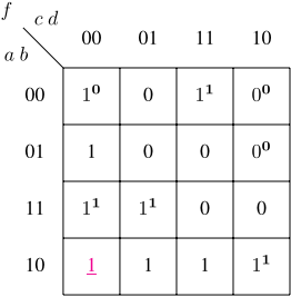
As soon as k > 0, the existence of a k-anchored abductive explanation for x given f and Σ is not ensured in general. Thus, on the previous example, x has no 3-anchored abductive explanation given f and Σ.
In the general case, deciding whether an instance x has a k-anchored abductive explanation given f and Σ is at the second level of the polynomial hierarchy: 2
Proposition 1. Given a domain theory about X (represented by a propositional formula or a Boolean circuit Σ), a binary classifier f over X (represented by a propositional formula or a Boolean circuit), an instance x ∈ X, a set RC ⊆ X of reference instances and an integer k > 0, deciding whether an instance x ∈ X has a k-anchored abductive explanation given f and Σ is Σp2 -complete in the general case (and this complexity holds in the restricted case when f is represented by a random forest).
Most anchored abductive explanations Instead of considering that the value of the bound k to be used has been provided by the explainee, we can determine its maximal value via an optimization process. In that case, one is interested in generating abductive explanations for x among the most anchored ones:
Definition 3. Given a domain theory about X (represented by a propositional formula or a Boolean circuit Σ), a binary classifier f over X (represented by a propositional formula or a Boolean circuit), and an instance x ∈ X, a set RC of reference instances, and a non-negative integer k, a most anchored abductive explanation t for x given f and Σ is a k-anchored abductive explanation for x given f and Σ such that k is maximal (i.e., no k+1-anchored abductive explanation for x given f and Σ exists).
2 In the supplementary material, we identify some conditions that makes the problem "only" NP-complete. Those conditions are satisfied when f is a decision tree.
A straightforward observation is that since every instance x has a 0-anchored abductive explanation given f and Σ, every instance x also has a most anchored abductive explanation for x given f and Σ.
Example 2 (Example 1 cont'd). On the previous example, x has a unique most anchored abductive explanation given f and Σ, namely {a, c}, and this explanation is 2-anchored. It can be observed that {a, c} is a subset-minimal abductive explanation for x given f and Σ.
However, in the general case, it is not ensured that the most anchored abductive explanations for x given f and Σ are among the subset-minimal abductive explanations for x given f and Σ. This comes from the condition stating that no instance from RC classified by f in a different way than x can be covered by a k-anchored abductive explanation for x given f and Σ.
Example 3 (Example 1 cont'd). Considering the previous example, if (1, 0, 0, 1) was added to RC , none of the subsetminimal abductive explanations for x given f and Σ (i.e., {a, c}, {a, b}, and {c, d}) would be a 0-anchored abductive explanation for x given f and Σ: after such an update of RC , the most anchored abductive explanations for x given f and Σ would be {a, c, d} and {a, b, d} (those explanations are 1-anchored abductive explanations for x given f and Σ) but they are not among the subset-minimal abductive explanations for x given f and Σ.
Obviously enough, as a by-product of Proposition 1, the computation of a most anchored abductive explanation for x given f and Σ is Σ2p -hard in the general case. Indeed, once a most anchored abductive explanation t for x given f and Σ has been computed, one can decide in polynomial time for any k whether x has a k-anchored abductive explanation for x given f and Σ: it is enough to count the number max of instances of R+ C covered by t when f(x) = 1 (resp. the number max of instances of RC covered by t when f(x) = 0) and to compare max with k to determine whether x has a k-anchored abductive explanation for x given f and Σ. This is the case if and only if max ≥ k.
4 Computing Example-Based Explanations
We now show how to derive a subset-minimal most anchored abductive explanation for a given instance x given f and Σ. Our algorithm is based on linear search where more and more anchored explanations are successively looked for. Thus, the algorithm consists in looking first for an a-anchored abductive explanation with a = 1, and if such an explanation t is found, to remove redundant literals from it to derive a subsetminimal explanation tsmin; then one computes from tsmin the largest integer i such that tsmin is an i-anchored abductive explanation, and the algorithm resumes with a = i + 1.
Of course, an algorithm to compute a k-anchored abductive explanation for x given f and Σ for a fixed k can be easily derived as a by-product of the latter algorithm (it is enough to stop the linear search whenever a ≥ k). If subset-minimality is not requested, one can also not run the code that remove redundant literals, at least at the last step (for the previous steps, the shifts from a to i + 1 that are made possible via subset-minimization prove computationally useful in general for improving the linear search).
Let us first explain how to compute an a-anchored abductive explanation for x given f and Σ, where a is any positive integer. Our approach relies on a two-phase procedure reminiscent to the well-established Counter-Example Guided Refinement Abstraction (CEGAR) paradigm [Clarke et al., 2003]. Given a ∈ N∗ , our approach iteratively generates a candidate t and then tests whether t actually is an a-anchored abductive explanation given f and Σ. Each candidate t is derived from a model of a CNF formula Φ generated from x, RC , and k. By construction, when x is such that f(x) = 1 (resp. f(x) = 0), a candidate t is a term satisfying t ⊆ tx such that at least a instances of R+ C (resp. RC ) are covered while avoiding any instances from RC (resp. R+ C ) . For each candidate t generated, the verification process then checks whether t is an abductive explanation for x given f and Σ. Since each test corresponds to an instance of a coNP-problem, one uses an NP oracle to achieve each of them. The generation step is repeated until every candidate has been considered but none of them has been retained (this shows that no a-anchored abductive explanation for x given f and Σ exists) or a candidate that qualifies as an a-anchored abductive explanation for x given f and Σ has been found.
The CNF formula Φ used to characterize the candidates t is based on additional Boolean variables. For each ℓi ∈ tx such that var(ℓi) = xi (an element of X = {x1, . . . , xn}), a variable sℓi is introduced. For any model ω of Φ, sℓi is set to 1 in ω precisely when the literal ℓi ∈ tx belongs to the candidate t associated with ω. Let RxC be the subset of RC consisting of instances classified by f in the same way as x. We have RxC = R+ C when x is a positive instance and RxC = RC when x is a negative instance. New variables associated with elements of RxC are also considered. To be more precise, a variable px′ is introduced for each reference instance x′ from RxC . For any model ω of Φ, px′ is set to 1 in ω precisely when the candidate t associated with ω covers both x and x′ .
The CNF formula Φ consists of the conjunction of three CNF formulae (1), (2), and (3).
The CNF formula (1) is composed of binary clauses indicating how the variables sℓi (i ∈ [n]) and px′ (x′ ∈ RxC ) are connected. Basically, whenever px′ is set to 1, every literal ℓi belonging to tx but not to tx′ must be set to 0 in order to ensure that the candidates t to be considered cover both x and x′ . This is ensured by considering the clause ¬sℓi ∨ ¬px′ within (1), that forces sℓi to be set to 0 when px′ is set to 1.
The CNF formula (2) ensures that any candidate t covers at least a instances from RxC . Primarily, the cardinality constraint ∑x′∈RxC px′ ≥ a is considered, and this constraint is turned into a CNF formula using state-of-the-art encoding techniques, as presented in [Roussel and Manquinho, 2021].
Finally, for being a candidate, t must not cover any instance x′ from RC \ RxC . We have that t does not cover x′ when there is at least one literal ℓi ∈ tx such that ∼ ℓi ∈ tx′ and ℓi belongs to t. To implement this, for each x′ from RC \ RxC a clause consisting of all the selector variables sℓi associated with the literals ℓi such that ℓi ∈ tx and ∼ ℓi ∈ tx′ must be satisfied.
Example 4 (Example 1 cont'd). To avoid too heavy notations, let us index the instances fromRxC = R+ C as follows:
Suppose that a = 1. The formula Φ for the running example is then composed of the following clauses:
By construction, every model ω of Φ characterizes a candidate t that consists of the literals ℓi of tx such that ω(sℓi ) = 1. t covers at least a elements of RxC and no element of RC \RxC . If there is no such model ω, i.e., if Φ is unsatisfiable, then no a-anchored abductive explanation for x given f and Σ exists. In the remaining case, in order to determine whether t qualifies as a true a-anchored abductive explanation for x given f and Σ, we need to verify whether t |= Σ ⇒ f holds when f(x) = 1 (and whether t |= Σ ⇒ ¬f holds when f(x) = 0). This is equivalent to examining whether the formula Γ = t ∧ Σ ∧ ¬f is unsatisfiable when f(x) = 1 (and whether Γ = t ∧ Σ ∧ f is unsatisfiable when f(x) = 0). If this verification condition holds, i.e., if Γ is unsatisfiable, then t is an a-anchored abductive explanation for x given f and Σ. Accordingly, the algorithm may stop if a is considered by the explainee as sufficiently large (i.e., a has reached a preset bound k).
Clearly enough, the resulting explanation t is not guaranteed to be subset-minimal (it is not in general). If we are interested in deriving from t a subset-minimal a-anchored abductive explanation tsmin for x given f and Σ, a simple greedy algorithm can be used. This greedy algorithm consists in considering the literals ℓi of t in a specific order and to test iteratively whether (t \ {ℓi}) ∧ Σ ∧ ¬f is still unsatisfiable when f(x) = 1 (and whether (t \ {ℓi}) ∧ Σ ∧ f is still unsatisfiable when f(x) = 0). If this is the case and t \ {ℓi} does not cover any instance from RC \ RxC , literal ℓi can be definitely removed from t (i.e., in the algorithm, t is replaced by t \ {ℓi}), otherwise it is kept and it will be kept when the next literals of t will be processed. At the end, when all the literals belonging to t at start have been processed, the resulting term tsmin is a subset-minimal a-anchored abductive explanation for x given f and Σ. Note that there is no need to test that whether tsmin covers at least a elements of RxC since this is necessarily the case (tsmin is a subset of t, so that every instance covered by t also is covered by tsmin). Though it is guaranteed that tsmin is a subset-minimal a-anchored abductive explanation for x given f and Σ, it turns out that tsmin can be more than a-anchored, thanks to the removal of redundant literals that took place when computing it.
From tsmin, we can compute in linear time the number i of elements of RxC that are covered by tsmin. Thus, when the goal is to compute a most anchored abductive explanation for x given f and Σ, the algorithm may resume with a = i + 1 as the next bound to be tested. Whenever i > a, the corresponding shift in the linear search is useful to get rid of computationally expensive, yet useless steps.
Example 5 (Example 1 cont'd). Suppose that the model ω of Φ has been found, such that ω satisfies sa, ¬sb , sc, sd , ¬p1, ¬p2, p3, ¬p4. The corresponding candidate t = {a, c, d} is a 1-anchored abductive explanation for x given f and Σ.
Considering the literals of t in sequence as folllows a, c, d, the greedy algorithm tests first whether {c, d} is a 1-anchored abductive explanation for x given f and Σ. This is not the case since this term covers the instance (0, 0, 0, 0) from RC \ RxC . Thus, at the next iteration, the greedy algorithm tests whether {a, d} is a 1-anchored abductive explanation for x given f and Σ. This is not the case since this term covers the model (1, 1, 1, 0) of ¬f while f(x) = 1. At the following iteration, the greedy algorithm tests whether {a, c} is a 1anchored abductive explanation for x given f and Σ. The test succeeds, so the subset-minimal explanation tsmin = {a, c} is returned.
Finally, one can realize that tsmin actually is a 2-anchored abductive explanation for x given f and Σ since it covers not only the instance (1, 1, 0, 0) from R+ C (just as the candidate t = {a, c, d} one started with), but also the instance (1, 1, 0, 1) from R+ C . Thus, once tsmin has been identified, there is no need to resume the search while looking for a 2anchored abductive explanation for x given f and Σ, since such an explanation has already been identified. The next step is thus to consider whether a 3-anchored abductive explanation for x given f and Σ, which is not the case for the running example (so the algorithm stops and tsmin is returned).
Now, if the verification condition is not met, indicating that the candidate t is not a true a-anchored abductive explanation for x given f and Σ, we need to search for an alternative candidate. To be sure that the spurious candidate term t will not be considered again during the generation step, one needs to block it. This could be achieved by simply adding to Φ a clause composed of the complementary literals to those satisfied by the model ω of Φ that characterizes t. However, this approach would be rather inefficient as it requires the addition to Φ of very large clauses, and each clause eliminates only a single model of Φ. A more robust approach consists in adding to Φ a constraint asserting that any subset of the candidate term t cannot be a valid a-anchored abductive explanation for x given f and Σ. Thus, the next candidates must include at least one literal not belonging to t. This can be ensured by adding to Φ a single clause given by (4):
Example 6 (Example 1 cont'd). Assume that a = 1 and that at the first iteration, the model ω1 of Φ satisfying sa, ¬sb , ¬sc, ¬sd , ¬p1, p2, p3, p4 has been computed. The associated candidate t1 = {a} is s.t. Γ = t1 ∧⊤∧¬f ≡ a∧¬f is satisfiable, as {a, b, c, ¬d} is a model of Γ. Thus, the verification condition does not hold. t1 = {a} is deemed a spurious candidate, prompting the addition to Φ of the clause sb ∨sc ∨sd . At the second iteration, suppose that the model ω2 of Φ∧ (sb ∨ sc ∨ sd ) has been found, where ω2 satisfies sa, ¬sb , sc, ¬sd , ¬p1, ¬p2, p3, p4. The associated candidate is t2 = {a, c}. Since t2 ∧ ¬f is unsatisfiable, the verification condition holds, showing that t2 = {a, c} is a 1-anchored abductive explanation for x given f and Σ. The derivation from t2 of a subset-minimal 1-anchored abductive explanation for x given f and Σ via the greedy algorithm leads to keep t2 as a whole (t2 does not contain any redundant literal). Then we can count the number of elements of RxC that are covered by t2 and realize that t2 actually is a subset-minimal 2-anchored abductive explanation for x given f and Σ.
5 Experiments
We made some experiments is order to figure out how our algorithm for deriving subset-minimal most anchored abductive explanations scales up. We focused on binary classifiers f represented by random forests.
Experimental setup The empirical protocol we considered was as follows. We have focused on 14 datasets issued from three well-known repositories, namely OpenML1 (openml.org), UCI2 (archive.ics.uci.edu/ml/), and UCR3 (timeseriesclassification.com). Multi-class datasets (balance and arrowhead) have been converted into datasets for binary classification using the one-vs-one approach. Ten random forests have been learned per dataset using scikit-learn. All the hyperparameters have been set to their default values (100 trees per forest). Categorical features have been one-hot encoded. Numerical features, have been binarized on-the-fly by the random forest learning algorithm. A 10-fold cross validation process has been achieved. All the experiments have been conducted on a computer equipped with Intel(R) XEON E5-2637 CPU @ 3.5 GHz and 128 Gib of memory.
Table 1 summarizes information about the datasets used and the random forests learned. The first four columns give respectively the dataset name (with a superscript indicating the repository from which it comes), the number of features (#F), the number of instances (#I) and the average number of Boolean conditions (#V ) used in the 10 random forests. The fifth column (%L) indicates the percentage of instances of the dataset that are labelled as negative. Finally, the last column gives the mean F1-score of the forests that have been learned.
| Dataset | #F | #I | #V | %L | F1-score |
|---|---|---|---|---|---|
| balance2 compas1 breasttumor1 divorce2 cleveland1 wine3 arrowhead3 australian1 | 4 | 337 | 28.0 | 85 54 | 90.72(±2.09) 61.03(±2.23) |
| 11 | 6172 | 69.5 | |||
| 37 | 286 | 114.9 | 58 | 62.6(±10.63) | |
| 54 | 170 | 116.5 | 51 | 97.59(±3.9) | |
| 22 | 303 | 663.3 | 54 | 80.47(±6.83) | |
| 234 | 111 | 851.2 | 51 | 97.31(±4.22) | |
| 249 | 146 | 879.4 | 45 | 85.39(±10.56) | |
| 38 | 690 | 1564.0 | 56 | 85.92(±5.69) | |
| biodegradation1 dexter1 | 41 | 1055 | 5730.7 | 66 | 90.98(±2.1) |
| 20000 | 600 | 7892.9 | 50 | 93.38(±2.76) | |
| spambase2 gisette1 | 57 | 4601 | 15005.5 | 61 | 96.24(±0.48) |
| 5000 | 7000 | 24464.6 | 50 | 97.54(±0.6) | |
| mnist381 | 784 | 13966 | 32638.6 | 51 | 98.67(±0.41) |
| christine1 | 1636 | 5418 | 43587.5 | 50 | 71.34(±2.16) |
Our goal was to evaluate the algorithm for computing a subset-minimal most anchored abductive explanation, presented in Section 4. For each dataset and each random forest learned, a set RC of reference instances has been selected uniformly at random from the training set. The number of reference instances retained in RC varied to consider 5%, 10% or 20% of the instances. Several encodings of random forests into CNF formulae exist (e.g., [Audemard et al., 2020; Izza and Marques-Silva, 2021]), we used the one presented in [Audemard et al., 2022]. A domain theory has been considered connecting the non-independent Boolean conditions used in the forests. Ten instances picked up uniformly at random in the corresponding test set have been considered. Thus, a total number of 100 instances per dataset has been considered. For each of them, the algorithm presented in Section 4 has been run in order to compute a most anchored abductive explanation and the number k of reference instances it covers. The SAT solver glucose [Audemard and Simon, 2009] has been used to address the various (un)satisfiability tests encountered at each run. A timeout (TO) of 60s has been considered per instance.
Experimental results Table 2 synthesizes the empirical results. The three main columns gather the results obtained for the three percentages used (5%, 10%, and 20%). Each main column is divided into six parts. The number of instances x for which the time limit has been reached during the search for a 1-anchored explanation is given in columns kTO =0 . The number of instances x for which our algorithm has proved that no 1-anchored explanation exists is given by columns kT O =0 . The number of instances x for which our algorithm has found during the search an explanation that is at least 1anchored is given by columns k>0. Accordingly, we have kT O =0 +kTO =0 +k>0 = 100. Columns kAV G >0 indicate the mean number of reference instances covered by the most anchored explanation that has been derived before the time limit, provided that this number is > 0. Columns time give the mean runtime (in seconds) used to compute a most anchored explanation when found before the time limit, and columns TO indicate the number of timeout (out of 100) that have been reached before the normal termination of the algorithm (i.e., when a subset-minimal most anchored explanation for x has been computed).
| Dataset | 5% | 20% | |||||||||||||||
|---|---|---|---|---|---|---|---|---|---|---|---|---|---|---|---|---|---|
| kT O =0 | kTO =0 k>0 | kAVG >0 | time | TO | kTO =0 | kTO =0 | k>0 | 10% kAVG >0 | time | TO | kTO =0 | kTO =0 | k>0 | kAVG >0 | time | TO | |
| balance | 0 | 8 | 92 4.9(±2.0) | 0.1(±0.0) | 0 | 0 | 2 | 98 | 9.2(±3.9) | 0.1(±0.0) | 0 | 0 | 0 | 100 | 17.9(±6.6) | 0.1(±0.0) | 0 |
| compas | 0 | 50 | 50 6.3(±6.6) | 0.2(±0.1) | 0 | 0 | 52 | 48 | 6.6(±4.8) | 0.3(±0.1) | 0 | 0 | 68 | 32 | 8.6(±6.0) | 0.6(±0.1) | 0 |
| breasttumor | 0 | 34 | 66 1.7(±0.9) | 0.2(±0.3) | 0 | 0 | 24 | 76 | 2.5(±1.6) | 0.3(±0.3) | 0 | 0 | 12 | 88 | 3.6(±2.5) | 0.4(±0.5) | 0 |
| divorce | 0 | 0 | 100 5.3(±1.1) | 0.1(±0.0) | 0 | 0 | 0 | 100 | 14.8(±0.6) | 0.1(±0.0) | 0 | 0 | 0 | 100 | 32.8(±3.2) | 0.2(±0.0) | 0 |
| cleveland | 0 | 6 | 94 4.1(±1.6) | 1.5(±1.0) | 0 | 0 | 4 | 96 | 7.9(±3.2) | 2.9(±2.2) | 0 | 0 | 2 | 98 | 13.6(±6.0) | 6.2(±5.2) | 0 |
| wine | 0 | 26 | 74 1.9(±0.8) | 0.2(±0.1) | 0 | 0 | 14 | 86 | 2.6(±1.1) | 0.3(±0.1) | 0 | 0 | 6 | 94 | 3.8(±1.7) | 0.6(±0.5) | 0 |
| arrowhead | 0 | 18 | 82 2.8(±1.3) | 0.3(±0.1) | 0 | 0 | 18 | 82 | 6.2(±2.1) | 0.5(±0.2) | 0 | 0 | 18 | 82 | 11.5(±3.3) | 6.3(±4.8) | 0 |
| australian | 0 | 2 | 98 6.1(±2.1) | 44.1(±19.6) | 54 | 0 | 2 | 98 | 10.2(±4.2) | 53.0(±14.2) | 74 | 0 | 0 | 100 | 16.6(±8.3) | 55.7(±12.9) | 86 |
| biodegradation | 2 | 6 | 92 2.5(±1.4) | 40.8(±22.7) | 52 | 4 | 6 | 90 | 3.1(±1.6) | 51.3(±15.6) | 67 | 4 | 6 | 90 | 4.3(±2.1) | 59.8(±1.3) | 90 |
| dexter | 0 | 30 | 70 2.5(±1.9) | 14.3(±16.4) | 6 | 0 | 28 | 72 | 3.2(±2.3) | 33.1(±23.1) | 22 | 0 | 26 | 74 | 4.3(±3.2) | 51.4(±16.5) | 56 |
| spambase | 18 | 8 | 74 1.6(±0.9) | 60.0(±0.0) | 92 | 28 | 8 | 64 | 1.9(±1.3) | 60.0(±0.0) | 92 | 24 | 6 | 70 | 2.5(±1.6) | 58.7(±7.8) | 92 |
| gisette | 0 | 18 | 82 2.6(±0.7) | 60.0(±0.0) | 82 | 0 | 14 | 86 | 2.5(±0.7) | 60.0(±0.0) | 86 | 0 | 10 | 90 | 2.0(±0.6) | 60.0(±0.0) | 90 |
| mnist38 | 17 | 0 | 83 1.0(±0.2) | 60.0(±0.0) | 100 | 12 | 0 | 88 | 1.1(±0.3) | 60.0(±0.0) | 100 | 19 | 0 | 81 | 1.1(±0.3) | 60.0(±0.0) | 100 |
| christine | 5 | 90 | 5 1.0(±0.0) | 60.0(±0.0) | 10 | 14 | 86 | 0 | ---- | ---- | 14 | 73 | 27 | 0 | ---- | ---- | 73 |
The datasets in Table 2 are sorted according to their difficulty, assessed by the value of #V in Table 1, that appears strongly correlated to the performance of our algorithm, as reflected by columns time and TO. Looking at columns TO, it turns out that the optimal value of k has systematically been found (i.e., no timeout) for half the datasets, i.e., up to the arrowhead dataset whatever the percentage used, and the time needed to determine this optimal value was very short (columns time). Furthermore, with a single exception, our algorithm has been able to point out useful information about at least 72% of the instances (even when the algorithm did not terminate normally). Indeed, for many instances x (their numbers being given in columns kTO =0 ), the algorithm succeeded in showing that no k-anchored explanation (with k > 0) exists for x. For many other instances x (their numbers being given in columns k>0), the algorithm succeeded in showing that a k-anchored explanation (with k > 0) exists for x. It can be checked that the sum kTO =0 + k>0 exceeds 72 for each dataset, whatever the percentage used, except for christine when the percentage used was 20%. Finally, our experiments has shown that the datasets used exhibit a significant discrepancy as to the number of instances that only have 0-anchored explanations.
6 Other RelatedWork
Our notion of anchored explanations should not be confused with the notion of dataset-based abductive explanations (aka sample-based explanations) introduced recently in [Cooper and Amgoud, 2023]. The (weak) dataset-based abductive explanations for x given f as pointed out in [Cooper and Amgoud, 2023] correspond to the abductive explanations for x given f in the sense of Definition 1 provided that the sole instances that are feasible are those in RC. A strong point of (weak) dataset-based abductive explanations is that they can be identified, derived and minimized w.r.t. setinclusion, in polynomial time. Furthermore, their computation does not require to have a representation of the classifier f available (an oracle for computing f is enough, thus black-box classifiers can be taken into account). The main downside of such explanations is that their correctness is not guaranteed. For instance, considering Example 1 again, a subset-minimal dataset-based abductive explanation for x = (1, 0, 0, 0) is {a}. Indeed, when the two instances (1, 1, 1, 1) and (1, 1, 1, 0) are considered as impossible because they do not belong to RC, one may assume that the corresponding decisions for them is 1. However, this does not comply with the decisions produced by the classifier. Indeed, f((1, 1, 1, 1)) = f((1, 1, 1, 0)) = 0 showing that {a} does not properly explain the behaviour of the classifier f when it predicts a positive decision for x since f(x) = 1.
7 Conclusion and Perspectives
We have defined example-based abductive explanations suited to binary classifiers. We proved that deciding whether a k-anchored abductive explanation for an instance exists is at the second level of the polynomial hierarchy when k > 0, which precludes the existence of efficient algorithms for generating such explanations. Nevertheless, we designed a CEGAR-based algorithm to derive subset-minimal most anchored abductive explanations. To evaluate its performance in practice, we focused on binary classifiers represented by random forests. Empirical results showed that despite the intrinsically high complexity of the problem it solves, our CEGAR-based algorithm is practical enough for "mildly hard" datasets, i.e., those leading to random forests based on up to a thousand Boolean conditions.
Several perspectives for further research can be pointed out. Thus, we plan to improve our CEGAR-based algorithm. A way to do it consists, during the generation phase, in looking for candidates t such that the number of literals of tx belonging to t is as high as possible. That way, clause (4) added at the refinement phase would restrict the remaining part of the search space in a more drastic way. Candidates t could be generated using a time-efficient local search approach (in that case the maximality of the number of literals of tx belonging to t would not be ensured) or using a MaxSAT solver (in that case, the optimality would be guaranteed at the price of a generation phase that would be computationally more demanding). In addition, it would be interesting to evaluate the empirical performance of our CEGAR-based algorithm when other binary classifiers than random forests are used.
Acknowledgements
Many thanks to the anonymous reviewers for their comments and insights. This work has benefited from the support of the AI Chair EXPEKCTATION (ANR-19-CHIA-0005-01) and of the France 2030 MAIA Project (ANR-22-EXES-0009) of the French National Research Agency (ANR). It was also partially supported by TAILOR, a project funded by EU Horizon 2020 research and innovation programme under GA No 952215.
@inproceedings{ijcai2024p407,
  title     = {On the Computation of Example-Based Abductive Explanations for Random Forests},
  author    = {Audemard, Gilles and Lagniez, Jean-Marie and Marquis, Pierre and Szczepanski, Nicolas},
  booktitle = {Proceedings of the Thirty-Third International Joint Conference on
               Artificial Intelligence, {IJCAI-24}},
  publisher = {International Joint Conferences on Artificial Intelligence Organization},
  editor    = {Kate Larson},
  pages     = {3679--3687},
  year      = {2024},
  month     = {8},
  note      = {Main Track},
  doi       = {10.24963/ijcai.2024/407},
  url       = {https://doi.org/10.24963/ijcai.2024/407},
}
TY - CPAPER TI - On the Computation of Example-Based Abductive Explanations for Random Forests AU - Audemard, Gilles AU - Lagniez, Jean-Marie AU - Marquis, Pierre AU - Szczepanski, Nicolas T2 - Proceedings of the Thirty-Third International Joint Conference on Artificial Intelligence, IJCAI-24 PB - International Joint Conferences on Artificial Intelligence Organization PY - 2024 SP - 3679 EP - 3687 DO - 10.24963/ijcai.2024/407 UR - https://doi.org/10.24963/ijcai.2024/407 ER -Copied
Machine-readable versions of this paper, for tools and AI agents:





