
Cutting the Black Box: Conceptual Interpretation of a Deep Neural Net with Multi-Modal Embeddings and Multi-Criteria Decision Aid
Proceedings of the Thirty-Third International Joint Conference on Artificial Intelligence. Main Track. Pages 3669-3678.
https://doi.org/10.24963/ijcai.2024/406
Keywords
- Machine Learning: ML: Explainable/Interpretable machine learning
- Knowledge Representation and Reasoning: KRR: Preference modelling and preference-based reasoning
- Machine Learning: ML: Trustworthy machine learning
- Computer Vision: CV: Interpretability and transparency
Abstract
This paper tackles the concept-based explanation of neural models in computer vision, building upon the state of the art in Multi-Criteria Decision Aid (MCDA).
The novelty of the approach is to leverage multi-modal embeddings from CLIP to bridge the gap between pixel-based and concept-based representations. The proposed Cut the Black Box (CB2) approach disentangles the latent representation of a trained pixel-based neural net, referred to as teacher model, along a 3-step process. Firstly, the pixel-based representation of the samples is mapped onto a conceptual representation using multi-modal embeddings. Secondly, an interpretable-by-design MCDA student model is trained by distillation from the teacher model, using the conceptual sample representation. Thirdly, the alignment of the teacher and student latent representations spells out the concepts relevant to explaining the teacher model.
The empirical validation of the approach on ResNet, VGG, and VisionTransformer on Cifar-10, Cifar-100, Tiny ImageNet, and Fashion-MNIST showcases the effectiveness of the interpretations provided for the teacher models. The analysis reveals that decision-making predominantly relies on few concepts, thereby exposing potential bias in the teacher's decisions.
- [Adadi and Berrada, 2018] Amina Adadi and Mohammed Berrada. Peeking inside the black-box: A survey on ex- plainable artificial intelligence (xai). In IEEE Access, 2018.
- [Bahadori and Heckerman, 2021] Mohammad Taha Ba- hadori and David E. Heckerman. Debiasing concept-based explanations with causal analysis. ICLR, 2021.
- [Bodria et al., 2023] Francesco Bodria, Fosca Giannotti, Riccardo Guidotti, Francesca Naretto, Dino Pedreschi, and Salvatore Rinzivillo. Benchmarking and survey of expla- nation methods for black box models. KDD, 2023.
- [Bresson et al., 2020] Roman Bresson, Johanne Cohen, Eyke Hüllermeier, Christophe Labreuche, and Michèle Se- bag. Neural representation and learning of hierarchical 2- additive Choquet integrals. In IJCAI, 2020.
- [Brown et al., 2020] Tom B. Brown, Benjamin Mann, Nick Ryder, Melanie Subbiah, Jared Kaplan, Prafulla Dhari- wal, Arvind Neelakantan, Pranav Shyam, Girish Sastry, Amanda Askell, Sandhini Agarwal, Ariel Herbert-Voss, Gretchen Krueger, Tom Henighan, Rewon Child, Aditya Ramesh, Daniel M. Ziegler, Jeffrey Wu, Clemens Win- ter, Christopher Hesse, Mark Chen, Eric Sigler, Ma- teusz Litwin, Scott Gray, Benjamin Chess, Jack Clark, Christopher Berner, Sam McCandlish, Alec Radford, Ilya Sutskever, and Dario Amodei. Language models are few- shot learners. In NeurIPS, 2020.
- [Bucila et al., 2006] Cristian Bucila, Rich Caruana, and Alexandru Niculescu-Mizil. Model compression. In KDD, 2006.
- [Carvalho et al., 2019] Diogo Carvalho, Eduardo Pereira, and Jaime Cardoso. Machine Learning Interpretability: A Survey on Methods and Metrics. In Electronics, 2019.
- [Chen et al., 2019] Chaofan Chen, Oscar Li, Chaofan Tao, Alina Jade Barnett, Jonathan Su, and Cynthia Rudin. This looks like that: Deep learning for interpretable image recognition. In NeurIPS, 2019.
- [Chen et al., 2020] Zhi Chen, Yijie Bei, and Cynthia Rudin. Concept whitening for interpretable image recognition. In Nature Machine Intelligence, 2020.
- [Chen et al., 2022] Qi Chen, Chaorui Deng, and Qi Wu. Learning distinct and representative modes for image cap- tioning. NeurIPS, 2022.
- [Choquet, 1953] G. Choquet. Theory of capacities. Annales de l'Institut Fourier, 1953.
- [Crabbé and van der Schaar, 2022] Jonathan Crabbé and Mi- haela van der Schaar. Concept activation regions: A generalized framework for concept-based explanations. NeurIPS, 2022.
- [Craven and Shavlik, 1995] Mark W. Craven and Jude W. Shavlik. Extracting tree-structured representations of trained networks. In NeurIPS, 1995.
- [Dargan et al., 2020] Shaveta Dargan, Munish Kumar, Maruthi Rohit Ayyagari, and Gulshan Kumar. A survey of deep learning and its applications: a new paradigm to machine learning. ACM in Engineering, 2020.
- [Dosovitskiy et al., 2020] Alexey Dosovitskiy, Lucas Beyer, Alexander Kolesnikov, Dirk Weissenborn, Xiaohua Zhai, Thomas Unterthiner, Mostafa Dehghani, Matthias Min- derer, Georg Heigold, Sylvain Gelly, Jakob Uszkoreit, and Neil Houlsby. An image is worth 16x16 words: Trans- formers for image recognition at scale. CoRR, 2020.
- [Fan et al., 2023] Wan-Cyuan Fan, Yen-Chun Chen, Dong- Dong Chen, Yu Cheng, Lu Yuan, and Yu-Chiang Frank Wang. Frido: Feature pyramid diffusion for complex scene image synthesis. AAAI, 2023. [Fel et al., 2023] Thomas Fel, Augusting Picard, Louis Bethune, Thibault Boissin, David Vigouroux, Julien Colin, Rémi Cadène, and Thomas Serre. Craft: Concept recursive activation factorization for explainability. CVPR, 2023.
- [Gilpin et al., 2018] Leilani H. Gilpin, David Bau, Ben Z. Yuan, Ayesha Bajwa, Michael Specter, and Lalana Kagal. Explaining explanations: An overview of interpretability of machine learning. In DSAA, 2018.
- [Goebel et al., 2018] Randy Goebel, Ajay Chander, Katha- rina Holzinger, Freddy Lecue, Zeynep Akata, Simone Stumpf, Peter Kieseberg, and Andreas Holzinger. Explain- able ai: The new 42? In Machine Learning and Knowledge Extraction, 2018.
- [Grabisch and Labreuche, 2010] M. Grabisch and Ch. Labreuche. A decade of application of the Choquet and Sugeno integrals in multi-criteria decision aid. Annals of Operation Research, 2010.
- [Grabisch, 1997] Michel Grabisch. K-order additive discrete fuzzy measures and their representation. Fuzzy Sets Syst., 1997.
- [Guidotti et al., 2018] R. Guidotti, A. Monreale, S. Ruggieri, F. Turini, F. Giannotti, and D. Pedreschi. A survey of methods for explaining black box models. ACM Comput- ing Surveys, 2018.
- [He et al., 2016] Kaiming He, Xiangyu Zhang, Shaoqing Ren, and Jian Sun. Deep residual learning for image recog- nition. In CVPR, 2016.
- [Herin et al., 2023] Margot Herin, Patrice Perny, and Na- taliya Sokolovska. Learning preference models with sparse interactions of criteria. IJCAI, 2023. IJCAI
- [Hessel et al., 2021] Jack Hessel, Ari Holtzman, Maxwell Forbes, Ronan Le Bras, and Yejin Choi. Clipscore: A reference-free evaluation metric for image captioning. In EMNLP, 2021.
- [Hinton et al., 2015] Geoffrey Hinton, Oriol Vinyals, and Jeff Dean. Distilling the knowledge in a neural network. In Deep Learning and Representation Learning Wshop, 2015.
- [Huang and Marques-Silva, 2023] Xuanxiang Huang and Joao Marques-Silva. The inadequacy of shapley values for explainability. CoRR, 2023.
- [Kim et al., 2018] Been Kim, Martin Wattenberg, Justin Gilmer, Carrie Cai, James Wexler, Fernanda Viegas, et al. Interpretability beyond feature attribution: Quantitative testing with concept activation vectors (tcav). In ICML, 2018.
- [Kingma and Ba, 2015] Diederik P. Kingma and Jimmy Ba. Adam: A method for stochastic optimization. In ICLR, 2015.
- [Koh et al., 2020] Pang Wei Koh, Thao Nguyen, Yew Siang Tang, Stephen Mussmann, Emma Pierson, Been Kim, and Percy Liang. Concept bottleneck models. In ICML, 2020.
- [Kusters et al., 2020] Ferdinand Kusters, Peter Schichtel, Sheraz Ahmed, and Andreas Dengel. Conceptual expla- nations of neural network prediction for time series. In IJCNN, 2020.
- [Labreuche and Fossier, 2018] Christophe Labreuche and Simon Fossier. Explaining multi-criteria decision aiding models with an extended shapley value. In IJCAI, 2018. IJCAI
- [Labreuche et al., 2016] Christophe Labreuche, Eyke Hüllermeier, Peter Vojtas, and Ali Fallah Tehrani. On the Identifiability of Models in Multi-Criteria Preference Learning. In DA2PL, 2016.
- [Lundberg and Lee, 2017] Scott M Lundberg and Su-In Lee. A unified approach to interpreting model predictions. NeurIPS, 2017.
- [Martyn and Kadziński, 2023] Krzysztof Martyn and Miłosz Kadziński. Deep preference learning for multiple criteria decision analysis. EJOR, 2023.
- [Miller, 1995] George A. Miller. Wordnet: A lexical database for english. In Communications of the ACM, 1995.
- [Molnar, 2020] Christophe Molnar. Interpretable machine learning. molnar, 2020.
- [Murdoch et al., 2019] W. James Murdoch, Chandan Singh, Karl Kumbier, Reza Abbasi-Asl, and Bin Yu. Definitions, methods, and applications in interpretable machine learn- ing. PNAS, 2019.
- [Paszke et al., 2019] Adam Paszke, Sam Gross, Francisco Massa, Adam Lerer, James Bradbury, Gregory Chanan, Trevor Killeen, Zeming Lin, Natalia Gimelshein, Luca Antiga, Alban Desmaison, Andreas Köpf, Edward Z. Yang, Zach DeVito, Martin Raison, Alykhan Tejani, Sasank Chilamkurthy, Benoit Steiner, Lu Fang, Junjie Bai, and Soumith Chintala. Pytorch: An imperative style, high- performance deep learning library. CoRR, 2019.
- [Radford et al., 2021] Alec Radford, Jong Wook Kim, Chris Hallacy, Aditya Ramesh, Gabriel Goh, Sandhini Agar- wal, Girish Sastry, Amanda Askell, Pamela Mishkin, Jack Clark, Gretchen Krueger, and Ilya Sutskever. Learning transferable visual models from natural language supervi- sion. ICML, 2021.
- [Ramesh et al., 2021] Aditya Ramesh, Mikhail Pavlov, Gabriel Goh, Scott Gray, Chelsea Voss, Alec Radford, Mark Chen, and Ilya Sutskever. Zero-shot text-to-image generation. In ICML, 2021.
- [Ribeiro et al., 2016] Marco Tulio Ribeiro, Sameer Singh, and Carlos Guestrin. "why should I trust you?" explain- ing the predictions of any classifier. In KDD, 2016.
- [Rozemberczki et al., 2022] Benedek Rozemberczki, Lau- ren Watson, Peter Bayer, Hao-Tsung Yang, Oliver Kiss, Sebastian Nilsson, and Rik Sarkar. The shapley value in machine learning. In IJCAI, 2022. IJCAI
- [Rudin, 2019] Cynthia Rudin. Stop explaining black box machine learning models for high stakes decisions and use interpretable models instead. Nature Machine Intelligence, 2019.
- [Saharia et al., 2022] Chitwan Saharia, William Chan, Saurabh Saxena, Lala Li, Jay Whang, Emily Denton, Seyed Kamyar Seyed Ghasemipour, Burcu Karagol Ayan, S. Sara Mahdavi, Rapha Gontijo Lopes, Tim Salimans, Jonathan Ho, David J Fleet, and Mohammad Norouzi. Photorealistic text-to-image diffusion models with deep language understanding. In NeurIPS, 2022.
- [Samek et al., 2022] Wojciech Samek, Grégoire Montavon, Andrea Vedaldi, Lars Kai Hansen, and Klaus-Robert Muller, editors. Explainable AI: Interpreting, Explaining and Visualizing Deep Learning. 2022.
- [Selvaraju et al., 2017] Ramprasaath R Selvaraju, Michael Cogswell, Abhishek Das, Ramakrishna Vedantam, Devi Parikh, and Dhruv Batra. Grad-CAM: Visual Explanations From Deep Networks via Gradient-Based Localization. In ICCV, 2017.
- [Simonyan and Zisserman, 2015] Karen Simonyan and An- drew Zisserman. Very deep convolutional networks for large-scale image recognition. In ACPR, 2015.
- [Sobrie et al., 2016] Olivier Sobrie, Mohammed El Amine Lazouni, Saïd Mahmoudi, Vincent Mousseau, and Marc Pirlot. A new decision support model for preanes- thetic evaluation. Computer Methods and Programs in Biomedicine, 2016.
- [Speer et al., 2017] Robyn Speer, Joshua Chin, and Cather- ine Havasi. Conceptnet 5.5: An open multilingual graph of general knowledge. In AAAI, 2017.
- [Tehrani et al., 2012] Ali Fallah Tehrani, Weiwei Cheng, Krzysztof Dembczyński, and Eyke Hüllermeier. Learn- ing monotone nonlinear models using the choquet integral. Machine learning, 2012.
- [Wang et al., 2021] Jiaxuan Wang, Jenna Wiens, and Scott Lundberg. Shapley flow: A graph-based approach to in- terpreting model predictions. In AISTATS, 2021.
- [Winter, 2001] E. Winter. The Shapley value, 2001.
- [Xiao et al., 2017] Han Xiao, Kashif Rasul, and Roland Vollgraf. Fashion-mnist: a novel image dataset for bench- marking machine learning algorithms. 2017.
- [Yuksekgonul et al., 2023] Mert Yuksekgonul, Maggie Wang, and James Zou. Post-hoc concept bottleneck methods. ICLR, 2023.
- [Zopounidis et al., 2015] Constantin Zopounidis, Emilios Galariotis, Michael Doumpos, Stavroula Sarri, and Kostas Andriosopoulos. Multiple criteria decision aiding for fi- nance: An updated bibliographic survey. EJOR, 2015.
References were extracted automatically from the PDF and may contain errors.
Full text extracted automatically from the PDF; figures, tables and equations may differ. The PDF is the version of record.
1 Introduction
Deep Neural Network (DNN) models, renowned for their impressive performance across various domains [Dargan et al., 2020], involve large and complex neural architectures. However, black-box models undermine user confidence in their results [Rudin, 2019]. The growth of the explainable AI (XAI) field [Craven and Shavlik, 1995; Kim et al., 2018; Goebel et al., 2018; Carvalho et al., 2019; Molnar, 2020; Samek et al., 2022; Bodria et al., 2023] is motivated by the fact that explaining DNNs is crucial to trusting, debugging or certifying them.
Given a DNN f, the state of the art in XAI aims to explain its outcome f(x) for any particular sample x (posthoc explanation) or explain f itself. Three main directions have been considered in the literature (Section 2). Along a first direction, the model is explained from the features most contributing to the decision (determined from the gradient of f(x) [Ribeiro et al., 2016] or from Shapley values [Lundberg and Lee, 2017; Wang et al., 2021]), and visualized through e.g. saliency maps [Selvaraju et al., 2017]. A second direction leverages external information on the application domain, represented through concepts and illustrative samples thereof, and searches for the impact of these concepts in the latent space of the model [Kim et al., 2018]. A third direction aims to characterize sample patterns generally associated with a class [Chen et al., 2019; Fel et al., 2023].
Independently, the field of Multi-Criteria Decision Aid (MCDA) has long been interested in characterizing and developing models for high-stakes decision-making. MCDA models are transparent-by-design, and they are meant to capture sophisticated decision preferences and strategies from experts / users [Zopounidis et al., 2015; Bresson et al., 2020]. It is fair to say that such models hardly deal with low-level, highdimensional representations.
The approach presented in this paper, called Cut the Black Box (CB2), aims to leverage the strengths of both DNN and MCDA fields in computer vision. 1 CB2 builds upon multimodal embeddings that map textual and visual information on the same real-valued representation [Radford et al., 2021; Ramesh et al., 2021; Saharia et al., 2022]. Such multi-modal embeddings, made public, are so efficient that they come to be used to define new evaluation metrics [Hessel et al., 2021; Chen et al., 2022; Fan et al., 2023]. The Contrastive Language-Image Pre-training (CLIP) embeddings [Radford et al., 2021], trained to align related textual and visual information, are used in this paper.
CB2 is a three-stage process (Section 3). In the first step, CLIP embeddings are used to map pixel-based samples into a conceptual space derived from a dictionary of the application domain. In the second step, the trained DNN model, called teacher model, is used to train, by distillation [Bucila et al., 2006; Hinton et al., 2015], a student model, which is an MCDA model built on the conceptual representation. In the third step, the intermediate concepts of the student model are aligned with the latent space of the teacher model: this alignment cuts the black box in the sense that they explain the similarity of two examples (and their same label) w.r.t. the teacher latent space from the concepts involved in these examples.
1 Code available at https://github.com/natixx14/CB2
The behavior of CB2 is studied experimentally in Section 5. Three black-box teacher models representative of various neural architectures are considered: ResNet [Simonyan and Zisserman, 2015], VGG [He et al., 2016] and VisionTransformer [Dosovitskiy et al., 2020]. Student models are trained from these teachers on the Cifar-10, Cifar-100, Tiny ImageNet and Fashion-MNIST benchmarks. Performance indicators include the difference in predictive accuracy between the teacher and student models and the alignment quality between their latent spaces. The explanation provided by CB2 is evaluated qualitatively based on the three or four main concepts associated with each class, and its sensitivity to the dictionary related to the application domain is examined. The paper concludes by discussing the approach's limitations and presenting some perspectives for further research.
Notations. The training set is denoted D = {(xi, yi), i = 1 . . . n}, where xi ∈ RD denotes the real-valued pixel-based representation of the i-th sample, and yi ∈ {1, . . . ,L} the associated class. The latent representation associated with a trained neural network is defined as its penultimate hidden layer of dimension d, denoted z.
2 RelatedWork
After a brief overview of the XAI domain, this section introduces the field of MCDA for the sake of self-containedness.
XAI. The state of the art in the rapidly evolving field of XAI [Craven and Shavlik, 1995; Lundberg and Lee, 2017; Goebel et al., 2018; Adadi and Berrada, 2018; Ribeiro et al., 2016; Gilpin et al., 2018; Carvalho et al., 2019; Murdoch et al., 2019; Molnar, 2020; Samek et al., 2022; Bodria et al., 2023] is briefly discussed, focussing on the approaches most related to CB2. As said, one of the main directions in XAI relies on external resources involving concepts related to the application domain and examples illustrating these concepts. This direction is pioneered by the Concept Activation Vector (CAV) framework [Kim et al., 2018]. Considering a given black box model f and its latent representation z, a specific concept such as 'striped' is associated with a classifier learned from the given positive and negative examples of 'striped', expressed using the latent z representation. The sensitivity of f to the 'striped' concept is evaluated by calculating how the classification of a training sample (e.g. 'zebra') is affected on average by intervening on this sample to make it 'less striped'. This process enables us to measure the causal effect of the concept 'striped' on the 'zebra' prediction.
Extensions have been proposed to overcome the limitations of CAV. [Crabb´e and van der Schaar, 2022] relax the assumption of linear classifiers using the kernel trick. [Bahadori and Heckerman, 2021] incorporate a causal prior graph to account for confounding factors and provide debiased interpretations. [Kusters et al., 2020] extend the approach to time series data. Overall, the main limitation of CAV seems to be the set of domain concepts potentially relevant to explain f and the existence of positive and negative examples for each concept. Another limitation is that CAV establishes that certain concepts are necessary to identify a given class (showing that zebra's probability decreases when the stripe property disappears). However, it does not guarantee that these concepts are sufficient to establish the prediction; we shall come back to this question in Section 5.1.
Another important direction in XAI has been proposed by [Chen et al., 2020], which disentangles latent representation using the so-called concept whitening (CW) operator. Like CAV, this approach assumes the definition of a set of potentially relevant low-level concepts (e.g. 'blue background' and 'silver objects') and the availability of samples illustrating each concept. CW is used to decorrelate and normalize the latent representation by aligning it with the axes corresponding to the concepts. This makes it interpretable insofar as the z coordinates reflect the importance of the concepts, e.g. the 'airplane' class is seen as linked to 'silver objects' on a 'blue background'. Building on conceptual bottleneck methods [Koh et al., 2020], the Post-hoc Concept Bottleneck Method alleviates the need for concepts and their associated samples by transferring concepts from other datasets or natural language concept descriptions via multimodal models [Yuksekgonul et al., 2023].
A third type of approach, proposed by [Fel et al., 2023], aims to characterize the patterns associated with a class visually. It involves cropping sub-images of the training samples, rescaling them and clustering them based on their Euclidean distance in the model latent space z. These clusters are considered to correspond to typical patterns of the class (e.g., the beak of a bird). The label predicted for an image is then explained from the clusters visited by its sub-images.
Multi-Criteria Decision Aid. In high-stakes decisionmaking fields, models are developed to help human users make decisions; nevertheless, human users must have the final say on these decisions. Transparent models are, therefore, needed to enable users to assess the extent to which the current case corresponds to the model's premises. Given the high-level descriptive characteristics, specific formalisms have been developed to express these transparent and consistent models, either designed in collaboration with domain experts or learned from data [Sobrie et al., 2016; Martyn and Kadzi´nski, 2023]. The approach presented focuses primarily on Choquet's integral formalism [Choquet, 1953] that can be learned from data [Tehrani et al., 2012; Herin et al., 2023]. Specifically, CB2 is built upon its hierarchical extensions (HCI; more in 3.2) for their properties of monotonicity and Lipschitz continuity, facilitating model interpretation. As [Bresson et al., 2020] shows, neural architectures can be defined so that the neural search space coincides with 2-additive HCIs, when the hierarchical structure is known. Even more interestingly, the HCI formalism can be used to calculate the Shapley value measuring the impact of any particular feature on the final decision, using a closedform expression [Labreuche et al., 2016]. Note that Shapley values are also used in XAI to explain a class from the features with the best Shapley values [Lundberg and Lee, 2017; Wang et al., 2021; Rozemberczki et al., 2022]. 2
Discussion. The key problem in the interpretation of blackbox models in computer vision can be seen as an grounding problem: even though the explanation sought can be formulated in terms of concepts ('striped', 'blue background'), these concepts must be linked to the internal representation of the model. In [Kim et al., 2018; Chen et al., 2020], these concepts are defined a priori and illustrative examples are provided; their grounding is formulated using classifiers learned at the top of z. In [Fel et al., 2023], the grounding problem is overcome by forming clusters from sub-images, using Euclidean distance based on z; these clusters can be visualized instead of named. In the MCDAmethods, the grounding problem is assumed to be solved before the learning phase, i.e. learning examples are directly expressed using the relevant concepts. The proposed approach aims to reconcile the above trends: multimodal embeddings map the pixel-based sample representation onto a conceptual one, addressing the grounding problem. An MCDA model, learned by distillation on the top of this conceptual representation, is aligned with the black-box teacher model and makes it possible to inspect the latent representation of the teacher. The proposed approach aims to reconcile the approaches mentioned: multimodal embeddings map the pixel-based representation of the sample into a conceptual representation, thus solving the grounding problem. It is also aligned with the teacher's latent representation and thus enables the inspection of the teacher's support for decisions. An MCDA model is built on this conceptual representation by distilling the black-box teacher. It is also aligned with the teacher's latent representation, enabling inspection of the elements leading the teacher to a decision.
2 After [Huang and Marques-Silva, 2023], the use of Shapley values in the XAI context is irrelevant when the target concept is best explained by the absence of a property. However, this limitation is of little importance in computer vision.
3 Overview of CB2
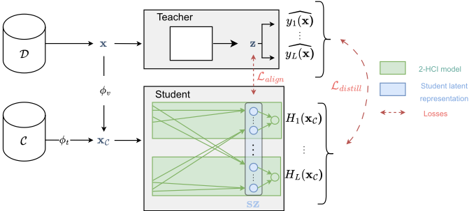
As indicated, CB2 is a three-step process (Fig. 1): 1, Pixelbased training samples are transposed into a conceptual representation (Section 3.1). 2, Using this representation, an MCDA model of the student is learned by distillation from the teacher model (Section 3.2). By design, this model enables the impact of each concept on the model's results to be characterized in closed form (Section 3.3). 3. The student's model is aligned with the teacher's model, enabling the teacher's latent to be interpreted through the student's transparent latent (Section 3.4).
3.1 Conceptual Representation
A set of K concepts C = {c1, . . . , cK} relevant to the application domain is selected a priori; class names are excluded to avoid tautological explanations. The sensitivity of the approach to the choice of C will be examined in Section 5.
Like [Yuksekgonul et al., 2023], CB2 performs grounding of selected concepts using multi-modal embeddings (as opposed to exploiting ad hoc samples representative of each concept and using them to learn a classifier hc on the top of the latent representation z as in [Kim et al., 2018]).
Specifically, we use a publicly available instance of the CLIP model [Radford et al., 2021], made of two frozen mappings denoted ϕv and ϕt, that respectively map visual and textual information on the same pivotal representation space Rm (ϕv : RD ↦→Rm; ϕt : text ↦→Rm). These mappings are trained using massive data formed of pairs (image x, caption y) by optimizing the alignment of ϕv(x) and ϕt(y).
The conceptual representation of a sample x ∈ RD , denoted xC, is defined as a real vector of dimension K, whose i-th coordinate expresses the relevance of the concept ci for image x:
As suggested in [Radford et al., 2021], xC is standardized using a softmax so that its coordinates are positive and the sum equals 1.
3.2 The MCDA Student Model
In MCDA, the (normalized) value of each attribute is interpreted as the utility of this attribute, or criterion score, for the sample. The overall utility of the sample, or sample preference score, is obtained by aggregating the criteria scores. The aggregation function is monotonic w.r.t. each criterion (the higher the score, the better the utility). The conceptual representation corresponds well to the MCDA framework by considering the i-th coordinate of xC (Eq. 1) as the 'utility' of concept ci for the sample x.
In this paper, the selected MCDA model space is that of 2-additive hierarchical Choquet integrals (2-HCI, detailed below) for the sake of their representational power and because they can be learned using back-propagation [Bresson et al., 2020].
Definition 1 (2-additive Choquet integral [Grabisch, 1997]). A 2-additive Choquet Integral function CI on Rk associates to each sample u = (u1, . . . , uk) ∈ Rk the sum of the pairwise aggregations of its coordinates ui:
parameterized from its weights ai, bi,j, ci,j. The fact that these weights are positive and sum to 1 guarantees that CI(u) is monotonic and lies in [0, 1] for u ∈ [0, 1]k .
A 2-additive Choquet integral, can represent two types of interaction between criteria Eq. (2): complementarity (both criteria must be well satisfied to produce a contribution, represented by a min function) and substitutability (it suffices for one of the two criteria to be well satisfied to produce a contribution, represented by a max function) [Grabisch and Labreuche, 2010].
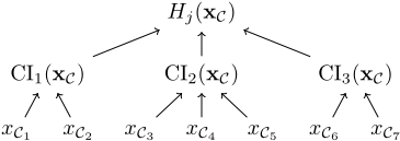
The 2-HCI function is defined as a 2-layer tree-structured connection graph (Fig. 2), where each node is a Choquet integral function. 3 Each CI node produces the aggregation of its children nodes, and the tree root node denoted H produces the global result.
The CB2 MCDA student model takes xC as input, where each coordinate xC,i reflects the relevance of concept ci for x. It involves L 2-HCI models, where model Hj stands for the score of the j-th class (j = 1 . . .L). Hj involves a first layer made of CI nodes (each one aggregating the utility of its children) and produces an overall utility Hj(xC), interpreted as the utility of the j-th class for x.
3 In the MCDA literature, the connection graph specifying how the coordinates/utilities are gradually aggregated is defined from expert knowledge. InCB2, we consider a random, balanced treestructured connection graph.
This student model is learned by distillation of the teacher model, building on the fact that a neural network can exactly represent a k-dimensional CI Choquet function [Bresson et al., 2020]. Constraints on the weights (Eq. (2)) are satisfied by characterizing the weights ai, bi,j, ci,j as the softmax of a parameter θ of dimension k2 , and this parameter vector is optimized by gradient back-propagation, minimizing the distillation loss [Hinton et al., 2015]. Formally, models H1 to HL are jointly trained from the conceptual dataset DC = {(xi,C,̂ y(xi), i = 1 . . . n}, with ̂ y(xi) the vector of teacher logits for the i-th sample, using a cross-entropy loss:
where ̂ yj(xi) stands for the j-th logit output of the teacher for the i-th training sample. The set of all CI nodes in the MCDA student is denoted sz.
3.3 Interpretation in Closed Form
In the XAI litterature, one option is to explain the sample label based on the impact of each feature on the label (feature attribution) [Ribeiro et al., 2016; Guidotti et al., 2018]. Some authors use the Shapley values to estimate the feature impact [Lundberg and Lee, 2017; Wang et al., 2021]. Shapley values originate from Cooperative Game Theory (CGT), which is used to distribute the commonwealth gained by all players fairly; formally, the Shapley value associated with one player averages his contribution to any coalition of players he participates in.
The parameters of the Choquet integral can be expressed as a set in CGT form, so the Shapley value naturally provides the average importance of each variable in this model.
Definition 2 (Shapley value in a Choquet integral [Grabisch and Labreuche, 2010]). The Shapley value of the i-th feature in Choquet node CI, noted Shap(CI, i) is 0 if CI does not involve the i-th feature; otherwise, it reads :
In the context of a 2-HCI model, however, Shapley values might be inconsistent as the importance of a node is not necessarily the sum of the importance of its children [Labreuche and Fossier, 2018], and a preferred alternative is to use Winter values [Winter, 2001]. Formally, the Winter value associated with the i-th leaf node of the 2-HCI model Hj is defined as the product of the Shapley values of all nodes on the path from i to the root node of Hj (Fig. 2) [Labreuche and Fossier, 2018]:
where CI is the parent of node i in Hj.
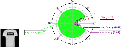
Visual Local Interpretation. A 2-additive Choquet integral can be visualized using a pie chart (Fig. 4b), where all slices represent all terms in Eq. (2): an individual term ui, or the complementarity min(ui, uj) between utilities ui and uj, or their substitutability termmax(ui, uj). The coefficient of the term (respectively ai, bi,j or ci,j) are depicted by the width of the slide.
3.4 Aligning the Teacher and the Student Models
The student model, trained from the teacher, reproduces its output by design. It remains, however, to ensure that the student delivers the same predictions as the teacher for the same reasons, that is, that the internal representation sz formed of all Choquet nodes consistently captures the same information as the latent representation z of the teacher.
This alignment is enforced by requiring a good approximation of z to be learned on the top of sz (being reminded that each node in sz is understandable by design). Likewise, a good approximation of sz is to be learned on the top of z, i.e. using an Auto-Encoder (AE) architecture (Fig. 1). The trained AE expresses each coordinate in z as a function of the Choquet nodes, thus disentangling this coordinate into the (few) concepts in the dictionary involved in these Choquet nodes.
Letting α and β respectively stand for the encoder and the decoder of the AE, the alignment loss is defined as:
3.5 CB2 Loss and Hyper-Parameters
Overall, the MCDA student model is learned by minimizing the sum of the distillation and the alignment losses. It is jointly trained with encoder α and decoder β using the compound loss:
where weights a and b are hyperparameters of the model.
As said, the importance of a concept for the teacher is assessed from the Winter values associated with this concept in the MCDA student. Interestingly, the bias of the teacher model can be inspected by a lesion study, comparing the student learned with the alignment (Eq. 7) and without the alignment (setting b = 0). If a concept is associated with a high Winter value for a class both with and without alignment, we conclude that this concept is both relevant and taken into account by the teacher. On the contrary, if the Winter value is higher with than without the alignment loss, the teacher may pay more attention to this concept than it should, and the expert might want to inspect for such discrepancies.
4 Experimental Setting
This section describes the experimental setting used to comparatively assess CB2. All experiments are performed on 8 Tesla V100 16GB GPUs. 4
4.1 Goals of Experiments
The aim of the experiments is to provide experimental answers to the following four questions:
- Q1: What are the relevant concepts to explain the teacher's classifications?
- Q2: How do these concepts differ from those used by the MCDA (transparent) student, i.e., is there a bias in the teacher's latent representation?
- Q3: How do the answers to the above questions depend on the set C of selected concepts (dictionary) ?
- Q4: How does the performance of theMCDA student compare with that of the teacher (due, for example, to the difference in representation and architecture)? Specifically, we are looking to see how well the student matches the teacher (making consistent predictions, regardless of accuracy) and how well it matches the ground truth labels of the samples.
4.2 Teachers, Datasets and Resources
Teachers. Three black-box teachers with different architectures are considered (Table 1): a ResNet [He et al., 2016], a VGG [Simonyan and Zisserman, 2015] and a visiontransformer [Dosovitskiy et al., 2020]. All models are pretrained on Imagenet and fine-tuned on each dataset. They are publicly available on the Pytorch hub [Paszke et al., 2019].
Datasets. Four well-known computer vision datasets are considered: Cifar-10, Cifar-100, Tiny Imagenet and FashionMNIST [Xiao et al., 2017]. Cifar-10 and Cifar-100 are used to compare CB2 explanations against the state of the art [Yuksekgonul et al., 2023]. Tiny Imagenet is used to evaluate the scalability of CB2 in relation to the number of classes and the diversity of concepts. Fashion-MNIST (black and white clothing images) is selected to evaluate the robustness of the CB2 approach when confronted with a different image distribution from CLIP. The standard training/test distribution is used for each dataset to train and test MCDA students.
Dictionary. The dictionary C is generally chosen by the expert [Kim et al., 2018; Koh et al., 2020]. In the experiments, two types of dictionary were selected for each dataset (set of classes): class-related concepts derived from the ConceptNet open-source ontology [Speer et al., 2017], augmented with the K most frequent nouns and adjectives from the English dictionary [Miller, 1995] (called COCA concepts); class-related concepts after a Large Language Model [Brown et al., 2020], mimicking common knowledge (called CK concepts). Class proper names and synonyms, as defined by WordNet, are removed from dictionaries to avoid tautological explanations (more details in code repository).
4 Further details are provided and included in the code repository at the following address https://github.com/natixx14/CB2.
| ResNet18 | Vgg | VitB16 | clipVitL14 |
| 64 | 512 | 284 | 768 |
4.3 CB2 Setting
Conceptual Representation. The CLIP embeddings [Radford et al., 2021] used to build the conceptual representation xC for each data sample x are a ViT-L/14 Transformer architecture for images and a masked self-attention Transformer for concepts. These embeddings, referred to as clipVitL14, are publicly available. 5
Learning the Student Model. The architecture of the student model (Fig. 2) is determined by the ℓ number of ICs, which governs the representational and explanatory power of each 2-HCI head. The implementation is carried out in PyTorch using the NeurHCI framework [Bresson et al., 2020]. The size of the transparent sz representation is ℓ × L, with L the number of classes. Alignment between the latent teacher and sz is achieved by an auto-encoder, implemented as a fully connected neural network (more details in code repository).
Hyper-Parameters. The learning criterion in CB2 (Eq. 7) involves three hyperparameters, respectively controlling the weight of the distillation term and the two reconstruction terms of the auto-encoder. The weights of these terms are determined by a grid search to obtain an optimal compromise between the adaptation of the teacher's result (distillation loss) and the teacher's latent representation (reconstruction loss). (see details in code repository). Learning hyperparameters (including the learning rate adapted using Adam [Kingma and Ba, 2015] and the patience determining search stop after a plateau) are also determined after a grid search (details of hyperparameter adjustment for each dataset and teacher are provided in the code repository).
4.4 Performance Indicators
Q1-Q2. For each class and dictionary, the concepts relevant to explaining the class are sorted according to their Winter values (Eq. 4). According to the teacher, the importance of the concept for a class is determined by training the MCA student using the global loss CB2 (Eq. 7). The potential bias in the teacher's treatment of the various concepts is assessed using a lesion study, comparing the initial Winter values with those obtained when training the MCDA student and setting the alignment weight to 0.
Q3. The impact of the dictionary is assessed by comparing the most influential concepts for each class (after their Winter value) and manually detecting whether any outlier concepts appear when considering the more general COCA dictionary rather than the CK dictionary.
5 https://huggingface.co/openai/clip-vit-large-patch14
Q4. The student is assessed by reporting: i) its faithfulness w.r.t. the teacher (the percentage of test samples where the student has the same label as the teacher); ii) its accuracy (the percentage of test samples where the student delivers the ground truth label). These performance indicators are compared with those reported by [Yuksekgonul et al., 2023] and those of a naive decision tree based on the conceptual representation for the Cifar-10 dataset.
5 Experimental Results
This section reports on and discusses the experimental results; further details are included in the code repository.
5.1 Conceptual Interpretation of Teacher Decisions
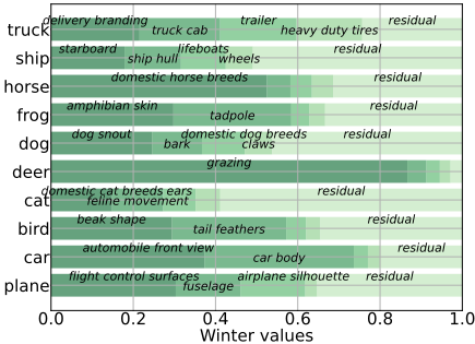
Global Explanation. Themodel is explained from the concepts with the highest Winter value (Eq. 5) for each class. For instance (Fig. 3), the truck class in Cifar-10 is explained from four concepts according to ResNet: delivery branding, truck cab, trailer and heavy-duty tyres, that together explain circa 75% of the decision. The area of the so-called residual rectangle, representing all the other concepts, measures the incompleteness of the explanation: the residual part for the deer class is less than 20% while it is circa 60% for the cat class.
Explanation also gives an indication of whether a prediction is sound or shallow. For example, the fact that the prediction deer is essentially supported by the concept grazing raises doubts as to whether the image of a deer on the beach will always be accurately classified.
Post-Hoc Explanation The decision for a given sample x can also be directly explained by the MCDA student. For instance, the MCDA model for the t-shirt class in Fashion-
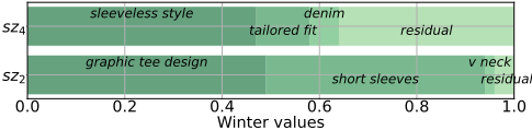
- (c) Explaining sz2 and sz4 with concepts' Shapley values.
Figure 4: Explaining teacher ResNet18 t-shirt prediction for instance x (a). The decision is explained in terms of latent aggregations sz, reporting their weights and their values for x (b). Finally, each sz can be explained and related with the concepts with top Shapley values (c).
MNIST reads (Fig. 4b):
with r(xC) corresponding to the remaining terms of the Choquet integral, whose total contribution is insignificant (less than 1%). As indicated (section 3.3), this HCI can be visualized in the form of a pie chart (Fig. reffig:pie). The angle of each slice reflects the coefficient associated with the corresponding HCI term, and its radius indicates the associated score for the sample. Finally, the score Ht-shirt(xC) corresponds to the total filled surface of the pie, showing the decisive impact of sz2 ∨sz4 for the sample under consideration.
Such a graphical representation can be proposed for each 2-HCI and sz composing the MCDA student model.
5.2 Inspecting the Teacher Biases
The second aim of the experiments is to identify teacher bias. These are highlighted by a lesion study, comparing the difference in Winter value for the same concept depending on whether the student is aligned with the teacher or not. This lesion study is made possible because 2-HCI models are very stable; the variance of Winter values calculated from models learned during different runs (with same connection graphs) is very moderate.
As illustrated in Fig. 5 for three classes of Fashion-MNIST for the VGG and ViT teachers, for some concepts, the student alignment with the teacher model results in a higher Winter value (in blue), suggesting that the teacher might be overlooking this concept. For example VGG might be overlooking the waistband concept for the coat class. For some other concepts, the student alignment results in a lower Winter value (in orange), suggesting that the teacher might be underlooking the concept; for instance, ViT might be underlooking the sweater style for the pullover class.
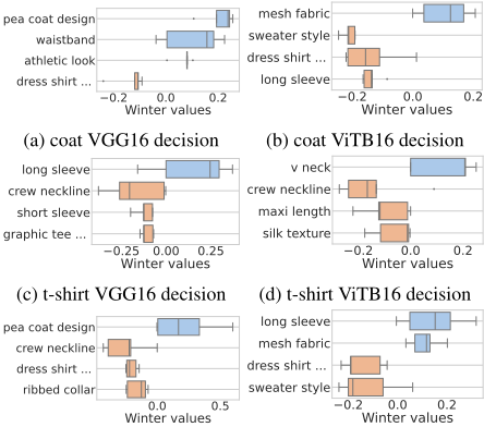
Figure 5: Inspecting the teacher biases w.r.t. three classes of Fashion-MNIST: (a)-(b): coat; (c)-(d): t-shirt; (e)-(f): pullover. Left: VGG teacher. Right: ViT teacher. In each case, the decision is linked to the concepts with top Winter value. In the case where the concept has more impact for the aligned student (and thus for the teacher) than for the non-aligned student, the positive difference is indicated with a blue box. In the opposite case, the negative difference is indicated with an orange box.
Overall, this lesion study highlights teacher reasoning biases, showing for example that the concepts v-neck and long sleeves are neglected by the ViT teacher for the prediction of the t-shirt and pullover classes respectively (Fig. 5). Conversely, screw neckline is not sufficiently taken into account by the teacher.
Interestingly, these results also enable users to select the models best suited to their interests. Typically, if an end-user is not interested in sleeve size when classifying shirts, he or she might opt for the Vision Transformer model rather than the VGG model.
5.3 Accuracy / Explainability Trade-Off and Impact of the Concept Dictionary
The predictions of the student model CB2 with the CK dictionary are evaluated on Cifar-10, comparing favorably with those of the teacher model ResNet, the state-of-the-art PCBM and PCBM-h baselines (results reported by [Yuksekgonul et al., 2023]) and a classical decision tree based on the same representation as the student (Table 2). The fact that the student outperforms the teacher is attributed to the quality of the CK dictionary and the fact that CLIP grounding is effective on Cifar-10 (as opposed to Fashion-MNIST see below).
An extract of the CB2 results, considering the four datasets, Cifar-10 0.77 ± 0.01
| PCBM CLIP concepts | PCBM-h CLIP concepts | CB2 Expert concepts | Decision tree Expert concepts | Teacher ResNet-18 | |
|---|---|---|---|---|---|
| Cifar-10 | 0.77 0.01 | 0.01 | 0.91 0.01 | 0.81 0.01 | 0.89 |
0.87± 0.01
0.91 ± 0.01
0.81 ± 0.01
| Model | Cifar-10 | Cifar-100 | Fashion-MNIST | Tiny ImageNet |
|---|---|---|---|---|
| random | 0.1 | 0.01 | 0.1 | 0.005 |
| ResNet-18 | 0.89 | - | 0.93 | - |
| CB2-R18-CK | 0.91 ± 0.01 | - | 0.56 ± 0.02 | - |
| CB2-R18-COCA | 0.37 ± 0.02 | - | 0.43 ± 0.01 | - |
| VGG | 0.85 | 0.43 | 0.91 | - |
| CB2-VGG-CK | 0.70 ± 0.07 | 0.10 ± 0.02 | 0.40 ± 0.02 | - |
| ViT-B-16 | 0.95 | 0.78 | 0.88 | 0.80 |
| CB2-ViTB16-CK | 0.85 0.04 | 0.27 0.02 | 0.47 0.03 | 0.21 0.01 |
CB2-ViTB16-CK 0.85 ± 0.04 0.27 ± 0.02
0.47 ± 0.03
0.21 ± 0.01
Table 3: Overall results for CB2 on Cifar-10, Cifar-100, FashionMNIST and Tiny ImageNet (columns 2 to 5), for teachers ResNet, VGG and ViT. For each teacher, student performance is indicated with the dictionary (CK or COCA). For comparison, the first row shows the accuracy of a random classifier, determined by the number of classes: 10 for Cifar-10 and Fashion-MNIST, 100 for Cifar-100 and 200 for Tiny ImageNet.
three teachers and two dictionaries, is given in Table 3. 6 As might be expected, the student's accuracy is highly dictionary-dependent: a huge performance loss (from 91% to 37%) is observed when considering the general purpose concepts (most common English nouns and adjectives; COCA dictionary) as opposed to the set of concepts associated with the classes after common knowledge (CK dictionary) on Cifar-10. The CB2 explanations also heavily depend on the dictionary: typically, a concept with very high Winter value for the cat class (and also for the dog class), though moderately informative, is the cute concept.
The student's performance also depends on the teacher and the size of its latent space: in the most favorable case (good teacher with a small latent space and few classes, i.e. ResNet on Cifar-10), the student outperforms the teacher. When the number of classes increases, as with Cifar-100 or Tiny ImageNet, the student's performance deteriorates considerably. This is due to the inadequacy of the dictionary, which is hardly capable of fine discrimination.
The student's poor performance on Fashion-MNIST is attributed to the CLIP image embedding, trained on a different distribution of images than Fashion-MNIST. It is interesting to note, however, that the student's lower predictive accuracy does not seem to affect the relevance of the explanations.
6 Conclusion and Perspectives
The Cut the Black Box approach aims to explain a teacher neural network by learning a surrogate student model. A first novelty compared to previous XAI approaches is that the student model uses a conceptual representation space, thanks to the multi-modal embeddings provided by CLIP [Radford et al., 2021]. A second novelty is that the student can be directly interpreted and visualized in terms of the concepts used in the dictionary, thanks to the Choquet integral formalism. 7
6 Only those pairs (dataset, teacher) for which the predictive accuracy is deemed satisfactory have been taken into account, in order to present meaningful results.
Experimental validation of CB2 shows the merits and limitations of the approach for various models and data sets. On the one hand, CB2 efficiently and quantitatively identifies a few concepts explaining the prediction of each class, according to their Shapley value. Interestingly, it also measures the proportion of the prediction explained by the concepts found; it can thus evaluate its performance autonomously.
One of the main limitations of the approach is that the relevance of the explanations depends on the dictionary considered and the multimodal embeddings. When considering a general-purpose dictionary, the explanations sometimes involve erroneous concepts reflecting the biases of the CLIP corpus (for example, linking the concept cute to the class cat). CB2 also encounters certain difficulties when the number of classes increases beyond a few dozen; the deterioration in performance is explained by the fact that more refined concepts would be required to discriminate between neighbouring classes.
The main research perspective opened up by CB2 is to autonomously find the dictionary of appropriate concepts, particularly in domains involving rare classes. A shorter-term perspective is to consider a more complex MCDA student model, for example by increasing the number of levels in the Choquet hierarchy and recovering stable concept associations during random variation of the hierarchical tree.
Acknowledgments
Christophe Labreuche has received support from the FaRADAI project (ref. 101103386) funded by the European Commission under the European Defence Fund (EDF-2021DIGIT-R). The work of Michele Sebag has been supported by the European Community under the Horizon 2020 programme: G.A. 952215 TAILOR.
Contribution Statement
Nicolas Atienza and Roman Bresson contributed equally to this work. This work was carried out when Roman Bresson was still at Thales Research and Technology.
@inproceedings{ijcai2024p406,
  title     = {Cutting the Black Box: Conceptual Interpretation of a Deep Neural Net with Multi-Modal Embeddings and Multi-Criteria Decision Aid},
  author    = {Atienza, Nicolas and Bresson, Roman and Rousselot, Cyriaque and Caillou, Philippe and Cohen, Johanne and Labreuche, Christophe and Sebag, Michèle},
  booktitle = {Proceedings of the Thirty-Third International Joint Conference on
               Artificial Intelligence, {IJCAI-24}},
  publisher = {International Joint Conferences on Artificial Intelligence Organization},
  editor    = {Kate Larson},
  pages     = {3669--3678},
  year      = {2024},
  month     = {8},
  note      = {Main Track},
  doi       = {10.24963/ijcai.2024/406},
  url       = {https://doi.org/10.24963/ijcai.2024/406},
}
TY - CPAPER TI - Cutting the Black Box: Conceptual Interpretation of a Deep Neural Net with Multi-Modal Embeddings and Multi-Criteria Decision Aid AU - Atienza, Nicolas AU - Bresson, Roman AU - Rousselot, Cyriaque AU - Caillou, Philippe AU - Cohen, Johanne AU - Labreuche, Christophe AU - Sebag, Michèle T2 - Proceedings of the Thirty-Third International Joint Conference on Artificial Intelligence, IJCAI-24 PB - International Joint Conferences on Artificial Intelligence Organization PY - 2024 SP - 3669 EP - 3678 DO - 10.24963/ijcai.2024/406 UR - https://doi.org/10.24963/ijcai.2024/406 ER -Copied
Machine-readable versions of this paper, for tools and AI agents:





