
Learning Preference Models with Sparse Interactions of Criteria
Proceedings of the Thirty-Second International Joint Conference on Artificial Intelligence. Main Track. Pages 3786-3794.
https://doi.org/10.24963/ijcai.2023/421
Keywords
- Uncertainty in AI: UAI: Decision and utility theory
- Knowledge Representation and Reasoning: KRR: Preference modelling and preference-based reasoning
- Machine Learning: ML: Learning preferences or rankings
Abstract
Multicriteria decision making requires defining the result of conflicting and possibly interacting criteria. Allowing criteria interactions in a decision model increases the complexity of the preference learning task due to the combinatorial nature of the possible interactions. In this paper, we propose an approach to learn a decision model in which the interaction pattern is revealed from preference data and kept as simple as possible. We consider weighted aggregation functions like multilinear utilities or Choquet integrals, admitting representations including non-linear terms measuring the joint benefit or penalty attached to some combinations of criteria. The weighting coefficients known as Möbius masses model positive or negative synergies among criteria. We propose an approach to learn the Möbius masses, based on iterative reweighted least square for sparse recovery, and dualization to improve scalability. This approach is applied to learn sparse representations of the multilinear utility model and conjunctive/disjunctive forms of the discrete Choquet integral from preferences examples, in aggregation problems possibly involving more than 20 criteria.
- [Adeyeba et al., 2015] Titilope A. Adeyeba, Derek T. Ander- son, and Timothy C. Havens. Insights and characteriza- tion of l1-norm based sparsity learning of a lexicographi- cally encoded capacity vector for the Choquet integral. In FUZZ-IEEE, pages 1 -7, 2015.
- [Ah-Pine et al., 2018] Julien Ah-Pine, Brice Mayag, and An- toine Rolland. Additive bi-capacity by using mathematical programming. In Third International Conference on Algo- rithmic Decision Theory (ADT), pages 15-29, 2018.
- [Anderson et al., 2014] Derek T. Anderson, Stanton R. Price, and Timothy C. Havens. Regularization-based learning of the Choquet integral. In FUZZ-IEEE, pages 2519 -2526, 2014.
- [Bach et al., 2012] Francis Bach, Rodolphe Jenatton, Julien Mairal, Guillaume Obozinski, et al. Optimization with sparsity-inducing penalties. Foundations and Trends® in Machine Learning, 4(1):1-106, 2012.
- [Beck, 2015] Amir Beck. On the convergence of alternating minimization for convex programming with applications to iteratively reweighted least squares and decomposition schemes. SIAM Journal on Optimization, 25(1):185-209, 2015.
- [Beliakov and Wu, 2019] Gleb Beliakov and Jian-Zhang Wu. Learning fuzzy measures from data: simplifica- tions and optimisation strategies. Information Sciences, 494:100-113, 2019.
- [Benabbou et al., 2017] Nawal Benabbou, Patrice Perny, and Paolo Viappiani. Incremental elicitation of Choquet ca- pacities for multicriteria choice, ranking and sorting prob- lems. Artificial Intelligence, 246:152-180, 2017.
- [Bresson et al., 2020] Roman Bresson, Johanne Cohen, Eyke Hüllermeier, Christophe Labreuche, and Michèle Se- bag. Neural representation and learning of hierarchical 2- additive Choquet integrals. In IJCAI, pages 1984-1991, 2020.
- [Chateauneuf and Jaffray, 1989] Alain Chateauneuf and Jean-Yves Jaffray. Some characterizations of lower probabilities and other monotone capacities through the use of möbius inversion. Mathematical social sciences, 17(3):263-283, 1989.
- [Daubechies et al., 2010] Ingrid Daubechies, Ronald De- Vore, Massimo Fornasier, and C Sinan Güntürk. Iteratively reweighted least squares minimization for sparse recov- ery. Communications on Pure and Applied Mathematics: A Journal Issued by the Courant Institute of Mathematical Sciences, 63(1):1-38, 2010.
- [de Oliveira et al., 2022] Henrique Evangelista de Oliveira, Leonardo Tomazeli Duarte, and João Marcos Travassos Romano. Identification of the Choquet integral parame- ters in the interaction index domain by means of sparse modeling. Expert Systems with Applications, 187, 2022.
- [Dyer and Sarin, 1979] James S Dyer and Rakesh K Sarin. Measurable multiattribute value functions. Operations re- search, 27(4):810-822, 1979.
- [Galand and Mayag, 2017] Lucie Galand and Brice Mayag. A heuristic approach to test the compatibility of a prefer- ence information with a choquet integral model. In Algo- rithmic Decision Theory -5th International Conference, ADT, pages 65-80, 2017.
- [Grabisch and Labreuche, 2010] Michel Grabisch and Christophe Labreuche. A decade of application of the Choquet and Sugeno integrals in multi-criteria decision aid. Annals of Operations Research, 175(1):247-286, 2010.
- [Grabisch et al., 2003] Michel Grabisch, Christophe Labreuche, and Jean-Claude Vansnick. On the extension of pseudo-boolean functions for the aggregation of interacting criteria. European Journal of Operational Research, 148(1):28-47, 2003.
- [Grabisch et al., 2008] Michel Grabisch, Ivan Kojadinovic, and Patrick Meyer. A review of methods for capacity iden- tification in Choquet integral based multi-attribute utility theory: Applications of the Kappalab R package. Eu- ropean journal of operational research, 186(2):766-785, 2008.
- [Grabisch et al., 2009] Michel Grabisch, Jean-Luc Marichal, Radko Mesiar, and Endre Pap. Aggregation functions, vol- ume 127. Cambridge University Press, 2009.
- [Grabisch, 1996] Michel Grabisch. The application of fuzzy integrals in multicriteria decision making. European jour- nal of operational research, 89(3):445-456, 1996.
- [Grabisch, 1997] Michel Grabisch. K-order additive discrete fuzzy measures and their representation. Fuzzy sets and systems, 92(2):167-189, 1997.
- [Grabisch, 2016] Michel Grabisch. Set functions, games and capacities in decision making. Springer, 2016.
- [Grandvalet, 1998] Yves Grandvalet. Least absolute shrink- age is equivalent to quadratic penalization. In Interna- tional Conference on Artificial Neural Networks, pages 201-206. Springer, 1998.
- [Herin et al., 2022a] Margot Herin, Patrice Perny, and Na- taliya Sokolovska. Learning sparse representations of preferences within Choquet expected utility theory. In The 38th Conference on Uncertainty in Artificial Intelligence, 2022.
- [Herin et al., 2022b] Margot Herin, Patrice Perny, and Na- taliya Sokolovska. Learning utilities and sparse represen- tations of capacities for multicriteria decision making with the bipolar Choquet integral. In Multidisciplinary Work- shop on Advances in Preference Handling, IJCAI, 2022.
- [Hüllermeier and Tehrani, 2013] Eyke Hüllermeier and Ali Fallah Tehrani. Efficient learning of classifiers based on the 2-additive choquet integral. In Computational Intelligence in Intelligent Data Analysis, pages 17-29, 2013.
- [Hurwicz, 1951] Leonid Hurwicz. The generalized bayes minimax principle: a criterion for decision making un- der uncertainty. Cowles Comm. Discuss. Paper Stat, 335:1950, 1951.
- [Jünger et al., 1993] Michael Jünger, Gerhard Reinelt, and Stefan Thienel. Practical problem solving with cutting plane algorithms in combinatorialoptimization. In Com- binatorial Optimization, 1993.
- [Kakula et al., 2020] Siva K Kakula, Anthony J Pinar, Tim- othy C Havens, and Derek T Anderson. Choquet integral ridge regression. In 2020 IEEE International Conference on Fuzzy Systems (FUZZ-IEEE), pages 1-8. IEEE, 2020.
- [Keeney et al., 1993] Ralph L Keeney, Howard Raiffa, and Richard F Meyer. Decisions with multiple objectives: pref- erences and value trade-offs. Cambridge university press, 1993.
- [Owen, 1975] Guillermo Owen. Multilinear extensions and the banzhaf value. Naval research logistics quarterly, 22(4):741-750, 1975.
- [Pelegrina et al., 2018] Guilherme D Pelegrina, Michel Gra- bisch, Leonardo T Duarte, and MT Romano. Multilinear model: New issues in capacity identification. In From Multiple Criteria Decision Aid to Preference Learning (DA2PL'2018), 2018.
- [Pelegrina et al., 2020] Guilherme Dean Pelegrina, Leonardo Tomazeli Duarte, Michel Grabisch, and João Marcos Travassos Romano. The multilinear model in multicriteria decision making: The case of 2-additive capacities and contributions to parameter identification. European Journal of Operational Research, 282(3):945- 956, 2020.
- [Pinar et al., 2017] Anthony J. Pinar, Derek T. Anderson, Timothy C. Havens, Alina Zare, and Titilope Adeyeba. Measures of the Shapley index for learning lower com- plexity fuzzy integrals. Granul. Comput., 2:303 -319, 2017.
- [Schmeidler, 1989] David Schmeidler. Subjective probabil- ity and expected utility without additivity. Econometrica, 57(3):571-587, 1989.
- [Shawe-Taylor et al., 2004] John Shawe-Taylor, Nello Cris- tianini, et al. Kernel methods for pattern analysis. Cam- bridge university press, 2004.
- [Tehrani and Hülermeier, 2013] Ali Fallah Tehrani and Eyke Hülermeier. Ordinal Choquistic regression. In EUSFLAT, 2013.
- [Tehrani et al., 2014] Ali Fallah Tehrani, Marc Strickert, and Eyke Hüllermeier. The choquet kernel for monotone data. In Esann, 2014.
- [Tehrani, 2021] Ali Fallah Tehrani. The choquet kernel on the use of regression problem. Information Sciences, 556:256-272, 2021.
- [Tibshirani, 1996] Robert Tibshirani. Regression shrinkage and selection via the lasso. Journal of the Royal Statistical Society. Series B (methodological), 58(1):267 -88, 1996.
- [Waegeman et al., 2009] Willem Waegeman, Bernard De Baets, and Luc Boullart. Kernel-based learning methods for preference aggregation. 4OR, 7(2):169-189, 2009.
- [Wakker and Deneffe, 1996] Peter Wakker and Daniel Den- effe. Eliciting von neumann-morgenstern utilities when probabilities are distorted or unknown. Management sci- ence, 42(8):1131-1150, 1996.
References were extracted automatically from the PDF and may contain errors.
Full text extracted automatically from the PDF; figures, tables and equations may differ. The PDF is the version of record.
1 Introduction
One of the main challenges of preference modeling in the context of multicriteria decision making is to construct simple and explainable decision models keeping sufficient flexibility to accurately model human preferences and decision behaviors. In the field of multiattribute/multicriteria decision making, the presence of possible interactions among criteria is a source of complexity for preference modeling because it prevents representing preferences by simple linear models such as weighted arithmetic means. More sophisticated weighted evaluation models including non-linear terms measuring the joint benefit or penalty attached to some groups of criteria are needed. Interactions may be represented by product terms as in the multilinear utility model [Keeney et al., 1993], or by minimum or maximum operations as in the Choquet integral [Grabisch et al., 2009], or possibly by other monotonic nonlinear factors involving several attributes or criteria.
∗ See http://www-desir.lip6.fr/∼perny/ijcai23/appendix.pdf for the proofs not included in the paper.
For example, if the decision maker (DM) prefers solutions with balanced utility vectors then one cannot simply use a weighted arithmetic mean of type ∑ni=1 wixi to define the overall utility attached to a utility vector (x1, . . . , xn). For instance, it would not be possible to make (0.5, 0.5) better than (1, 0) and (0, 1) simultaneously. A simple solution in this case may be to allocate a bonus to alternatives that perform well on all criteria. It is sufficient to add a conjunctive term to the weighted mean, e.g., ∏ni=1 xi or min{x1, . . . , xn}, weighted by a sufficiently large positive coefficient. We observe indeed that this conjunctive term takes a strictly positive value on (0.5, 0.5) but remains null on (1,0) and (0,1). More generally, beyond the linear part of the aggregation function, various interaction terms could be inserted to model positive but also negative synergies within some groups of criteria.
However, allowing the possibility of interactions in a decision model is a source of complexity in preference modeling and preference learning due to the combinatorial nature of these interactions. In an aggregation model involving n criteria, interactions may appear in any of the 2n - n - 1 subsets of criteria including more than one element. For n = 10 criteria it represents slightly more than 1000 possible interactions to analyze. When n = 20 it already represents more than one million possible interactions. In order to preserve scalability in learning the interactions, a standard approach is to reduce the combinatorial aspect of the problem by allowing only a limited number of them. For example one can just consider pairwise interactions of criteria. More generally one could limit interactions to subsets of size k for some k significantly smaller than n. However, this prior restriction eliminates very simple and natural representations of preferences that require larger interactions. For example, in the above example, we have shown that the introduction of a conjunctive term including all criteria may be natural to promote balanced solutions. Besides, another simple example is the Hurwicz criterion [Hurwicz, 1951] which is standardly used to make a tradeoff between the worst and the best components. It is defined as a convex combination of min{x1, . . . , xn} and max{x1, . . . , xn} and therefore includes two interactions terms. Both of them involve the entire set of criteria and cannot be simply approximated by interactions on smaller sets.
Here we would like to propose another approach where no prior restriction on the possible interaction groups is made. The useful groups will emerge from preference data with the aim of constructing a model as simple as possible, that fits well the preference examples. In this perspective, we consider an aggregation function defined as a weighted sum of factors made of criteria in interaction and propose a method to learn a sparse representation of these weights.
The paper is organized as follows: In Section 2 we recall some background on multicriteria aggregation models including interacting components. Then in Section 3 we introduce an approach to obtain sparse representations of interactions by iterative reweighted least square regularization, and dualization to improve the scalability of the approach. Section 4 presents some numerical tests to evaluate the performance of the proposed approach both in terms of computation time and generalizing performances.
2 EvaluationModels with Interacting Criteria
The general framework. In a multidimensional decision problem, the alternatives are described with respect to n points of views (n > 1) that must be considered in the evaluation process. Depending on the decision context, these viewpoints may refer to different attributes describing the alternatives (multiattribute decision making), different criteria used to compare the alternatives (multicriteria decision making), or different individuals expressing their preferences (multiagent decision making). In any case, every alternative x is described by a vector (c1(x), . . . , cn(x)) of consequences where ci(x) represents the value of x with respect to the ith viewpoint. Let N = {1, . . . , n} denote the index set of viewpoints. Let Xi denote the set of possible consequences on the ith viewpoint for all i ∈ N and X = X1 × . . . ×Xn the set of all possible consequence vectors. Let ≿ be the preference relation of the DM over X. One standard approach in preference modeling consists of representing ≿ by a decomposable function u on X of the form:
where ui : Xi → [0, 1], i ∈ N are marginal utility functions representing the attractiveness of consequences ci(x) for the DM and F : [0, 1]n → [0, 1] is an aggregation function nondecreasing in each argument. Function u is said to represent ≿ when x ≿ y if and only if u(x) ≥ u(y). Throughout the paper, ≻ is used to denote the asymmetric part (strict preference) of ≿ whereas ∼ denotes its symmetric part (indifference).
Let us recall two standard examples of function u, widely used to represent preferences in multiattribute/multicriteria decision problems involving criteria in interaction:
Example 1. The multilinear utility model defined by:
was introduced in the context of multiattribute decision making under risk [Keeney et al., 1993] but is also used and axiomatically justified in the context of multiattribute decision making [Dyer and Sarin, 1979] and [Grabisch, 2016, Chap.
6]. In the context of this paper, v is a set function defined on the power set 2N and valued in the unit interval, assigning a weight to any subset of viewpoints. Another well-known decision model defined from a set function v is the following:
Example 2. The discrete Choquet integral
where (.) is any permutation of N such that u(i)(c(i)(x)) ≤ u(i+1)(c(i+1)(x)) and X(i) = {(i), . . . , (n)}, i ∈ N with x(0) = 0 and X(n+1) = ∅. For instance, if n = 3 and x is such that u2(c2(x)) ≤ u1(c1(x)) ≤ u3(c3(x)), then Cv(x) = [v(1, 2, 3) - v(1, 3)]u2(c2(x)) + [v(1, 3) - v(3)]u1(c1(x)) + v(3)u3(c3(x)).
The Choquet integral was initially introduced in the context of decision making under uncertainty [Schmeidler, 1989] but is also widely used in the context of multiattribute/multicriteria decision making [Grabisch, 1996; Grabisch and Labreuche, 2010].
In both models (multilinear and Choquet), one can assume that v is normalized, i.e., it satisfies boundary conditions v(∅) = 0 and v(N) = 1. It is also generally assumed that v is monotonic with respect to set inclusion (which guarantees the monotonicity of u w.r.t. weak Pareto dominance). More formally, if v(A) ≤ v(B) for all subsets A, B ⊆ N such that A ⊆ B then ui(ci(x)) ≥ ui(ci(y)) for all i ∈ N implies u(x) ≥ u(y) for all pairs (x, y) whether u is defined by (2) or (3). Such monotonic set functions named capacities are widely used in preference aggregation [Grabisch et al., 2003; Grabisch, 2016]. The capacity provides a non-necessarily additive weighting system (the weight of a set is not necessarily the sum of the weights of its elements) and super-additivity and sub-additivity are used to model positive and negative synergies between the components of the decision model.
The capacity is a preference parameter that must be elicited by questioning the DM or learned from preference examples. The other preference parameters used in these models are marginal utility functions ui, i ∈ N that can be obtained before the identification of the capacity. In the case of the multilinear model, marginal utilities can be elicited using standard gamble queries under mutual utility independence, an axiom usually assumed to justify the multilinear model under uncertainty [Keeney et al., 1993]. They can alternatively be derived from comparisons of preference intensities under weak difference independence, an axiom usually assumed to justify the multilinear model in multicriteria/multiattribute decision making [Grabisch, 2016, Chap. 6]. For the Choquet integral, the utility functions can be obtained using standard sequences of tradeoff queries [Wakker and Deneffe, 1996], or constructed with the Macbeth method [Grabisch and Labreuche, 2010] or learned from preference examples [Herin et al., 2022b]. We assume here that functions ui have been elicited beforehand using one of the above mentioned methods and we focus on learning the capacity from preference examples. From now on, any alternative x is described by the utility vector x = (x1, . . . , xn) ∈ [0, 1]n where xi = ui(ci(x)), i ∈ N.
Respresentations based on M¨obius masses. A useful alternative representation of any capacity v is given by its M¨obius transformmv defined as follows:
The values mv(S) are called M¨obius masses. We remark that we necessarily have ∑T⊆N mv(T ) = 1, since v(N) = 1.
It is interesting to note that MLv(x) can be direclty defined fromM¨obius masses as follows [Owen, 1975]:
Similarly, Cv(x) admits several reformulations from mv [Chateauneuf and Jaffray, 1989; Grabisch et al., 2009]:
where ¯ v is the conjugate of v, i.e., the capacity defined by ¯ v(S) = v(N) - v(N \ S) for all S ⊆ N.
| S | 1 | 2 | 3 | 1, 2 | 1, 3 | 2, 3 | 1, 2, 3 |
| v(S) | 0.1 | 0.2 | 0.3 | 0.3 | 0.4 | 0.5 | 1.0 |
|---|---|---|---|---|---|---|---|
| mv(S) | 0.1 | 0.2 | 0.3 | 0.0 | 0.0 | 0.0 | 0.4 |
| ¯ v(S) | 0.5 | 0.6 | 0.7 | 0.7 | 0.8 | 0.9 | 1.0 |
| m¯ v(S) | 0.5 | 0.6 | 0.7 | -0.4 | -0.4 | -0.4 | 0.4 |
Let x = (x1, x2, x3) with x2 ≤ x1 ≤ x3. Then we have: MLv(x) = 0.1 x1 +0.2 x2 +0.3 x3 +0.4 x1x2x3 (Eq. 4) Cv(x) = 0.1 x1 +0.2 x2 +0.3 x3 +0.4 x2 (Eq. 5).
Here the disjunctive form of Cv (Eq. 6) is less interesting because m¯ v is less sparse than mv. The converse holds for C¯ v. We have C¯ v(x) = 0.1x1 + 0.2x2 + 0.3x3 + 0.4x3 by Eq. 6 whereas the conjunctive form based on m¯ v is less compact.
In order to factorize and generalize Equations 4-6, we will now consider a general decision model of the form:
where mS are M¨obius masses and ϕS aggregates the quantities xi, i ∈ S to define the interaction term ϕS(xS). Thus ϕS is the product if F is the multilinear model and ϕS is the min (resp. max) operation if F is the conjunctive (resp. disjunctive) form of the Choquet integral. Note that function F (x) reads as the following inner product F (x) = ⟨m, ϕ(x)⟩ where m = (mS)S⊆N and ϕ : Rn → R2n maps x into a nonlinear feature space: ϕ(x) = (ϕS(xS))S⊆N. Both vectors m and ϕ(x) are indexed by the subsets S ⊆ N numbered in lexicographic order.
M¨obiusmasses and interactions. Acapacity v is said to be k-additive if mv(S) ̸= 0 for some S of size k and mv(S) = 0 for all S of size greater than k [Grabisch, 1997]. When v is 1-additive, all interaction terms vanish and F boils down to a weighted arithmetic mean of components xi. When v is 2additive, only pairwise interactions are possible in the model (terms of type ϕij(xi, xj) in Equation 7). Their coefficients mv({i, j}) = v({i, j}) - v({i}) - v({j}) can be positive or negative and their magnitude measures the importance of the interaction between i and j (the gap to additivity).
It is frequently assumed that capacities are k-additive for some k < n prior to preference analysis so as to make sure that v admits a polynomial-size representation in terms of M¨obius masses. However, it strongly reduces the descriptive power of the ML and Choquet models. For example, the preference for balanced solutions mentioned in the introduction requires mv(N) > 0 (a bonus is given to alternatives that perform well on all criteria) which is incompatible with kadditivity for any k < n. In this case, a n-additive capacity is needed without any restriction on the size of possible interactions. Several measures of interaction have been proposed in the literature to measure the magnitude of interactions within sets of any size. For example, the Banzhaf and Shapley interactions indices IB(S) and ISh(S) associated to a subset S ⊆ N in models MLv and Cv are related to M¨obius masses mv as follows [Grabisch et al., 2009]:
We remark that these interaction indices tend to vanish as M¨obius masses tend to 0. Thus, favouring the sparsity of the M¨obius vector m in an aggregation function defined by Equation 7 tends to reduce the criteria interactions in the associated decision model.
Related work. As far as the identification of the capacity used in a decision model is concerned, several approaches based on the least squares criterion or variance minimization of the model under preference constraints have been proposed in the field of multicriteria analysis for the Choquet integral [Grabisch et al., 2008; Grabisch and Labreuche, 2010]. In the field of machine learning different learning algorithms have been proposed, e.g., Choquistic regression [Tehrani and H¨ulermeier, 2013], support vector machines (SVM) with Choquet kernel [Tehrani, 2021], and ridge regression for Choquet regression [Kakula et al., 2020]. Moreover a neural network was recently proposed to learn a hierarchical Choquet model [Bresson et al., 2020]. Active learning approaches also exists based on regret minimization [Benabbou et al., 2017]. Some recent contributions using regression also exist for the multilinear model [Pelegrina et al., 2018; Pelegrina et al., 2020].
The complexity of models involving capacities, having in general 2n - 2 free parameters, is prohibitive for many real-life applications. Very often, a prior complexity reduction is obtained by considering models with k-additive capacities (k = 2 being the most common choice) [Grabisch et al., 2008; H¨ullermeier and Tehrani, 2013; Galand and Mayag, 2017; Ah-Pine et al., 2018; Bresson et al., 2020; Pelegrina et al., 2020]. Similar restrictions exist for limiting interactions with the notion of k-interactivity [Beliakov and Wu, 2019].
A less restrictive and more flexible attempt to reduce models complexity is to derive a sparse representation of the capacity from preference data using the L1 penalty term [Anderson et al., 2014; Adeyeba et al., 2015; Pinar et al., 2017; de Oliveira et al., 2022] where the regularization was applied either to the capacity, or to the interaction index. Recently, some evidence was given that M¨obius representations often lead to more compact preference representations and an approach based on linear programming (LP) was proposed to learn a sparse M¨obius transform of the capacity in the Choquet integral [Herin et al., 2022a]. However the absence of prior restriction on capacities comes at the expense of computation times and scalability.
Our contribution in this paper is to propose a faster and more scalable algorithm to learn sparse M¨obius representations of capacities from preference examples, for the multilinear and Choquet models and any other instance of Eq. 7. Our approach relies on iteratively re-weighted least squares and dualization as explained in the next section.
3 ADual IRLS for Sparse Preference Learning
Our objective is to learn a sparse representation of m based on a training set of preferences statements {(xi , yi ) ∈ X 2 : xi ≻ yi , i ∈ P} and possibly of indifference statements {(xi , yi ) ∈ X 2 : xi ∼ yi , i ∈ I}. A well-known workhorse for learning sparse models is the L1-norm penalty. This is indeed a sparse-inducing penalty, in the sense that it promotes solutions with few non-null coefficients. A major application of this regularization is the LASSO estimate [Tibshirani, 1996] in linear regression. Then, our learning problem is to minimize both the error on the preference examples and the L1 norm of the M¨obius vector. The L1-penalization is only applied to the terms involving at least two criteria so as to minimize interactions. The approximation problem is thus formulated as follows:
where variable mj is the j th component of vector m. The hyper-parameter λ > 0 controls the level of regularization and δ is a strictly positive discrimination threshold used to separate preference from indifference situations. Variable ϵi models the positive error made on the preference example xi ≻ yi , while ϵ+i - ϵ-i models the signed error made on the indifference xi ∼ yi . The constraint m(∅) = 0 is implicit.
Problem P can be solved by linear programming using the following L1-norm linearization:
where variables w+ j ,wj are used for the linearization of |mj|. Despite a simple linearization, the obtained linear program still drags an exponential number of variables (2n (3 - 2n) + |P| + 2|I|) and thus is hardly solvable for more than a dozen of criteria. For the sake of scalability, we propose to solve P by solving a sequence of sub-problems Pk that admit an efficient dual formulation. More precisely, we use an iteratively reweighted least square (IRLS) algorithm [Daubechies et al., 2010; Bach et al., 2012; Beck, 2015; Grandvalet, 1998] that consists in approximating the solution of a L1-penalized problem with a sequence of least squares problems. Sparsity is recovered by increasingly penalizing non significant coefficients with a squared L2 regularization. The interest of this method lies in the fact that a least squares problem is easy to solve in general. In our case, we will show that the least square problemPk admits a compact dual form whose size is no longer exponential in n the number of criteria, but linear in |P |+|I|, the number of preference examples. More specifically, L1-optimization is linked to least squares problems through the quadratic variational formulation of the L1-norm [Bach et al., 2012] that allows absolute values to be expressed as infimums of weighted squared values:
Using Eq. 12, we now establish Proposition 1 providing an IRLS algorithm that approximatively solves P. The proof relies on the framework introduced in [Beck, 2015] that gives conditions under which an optimization problem can be solved by alternating minimization (here on m and z) and insights on how this algorithm can lead to IRLS sequences.
Proposition 1. Let η > 0 be a smoothing parameter. Consider the sequence m(k) initialized with m(0) = 1 such that:
s.t. (8), (9), (10), (11)
Then we have: limk→∞ J(m(k+1) )-J ∗ ≤ (2n -n)η where J is the objective function of P and J ∗ its optimum. Pk refers to the problem solved at each iteration.
Proof. Let η > 0 be a smoothing parameter and Pη the associated surrogate problem of P where the sum of absolute values is replaced by a differentiable term:
Remarking that ϵi = (δ - ⟨m, δi ⟩)+ and ϵ+i - ϵ-i = ⟨m, δi ⟩ at the optimum, where δi = ϕ(xi ) - ϕ(yi ) and (x)+ = max(0, x) , Pη can be reformulated in an unconstrained form:
with 1{⟨m,1⟩=1} = 0 if ⟨m, 1⟩ = 1 and +∞ otherwise. Then, introducing the smoothing parameter η in Eq.12 yields:
which leads to reformulate Pη as a problem involving two blocks of variables (m, z):
Since g1, g2 are closed proper convex functions subdifferentiable over their domains dom g1 and dom g2, and f is convex and continuously differentiable over dom g1 × dom g2 (and ∇zf Lispschitz continuous), this problem fits in the class of problem solvable by alternating minimization [Beck, 2015]. Applied on problem Pη and initialized at m(0) this algorithm is:
A proof of a non asymptotic sublinear convergence rate of the alternating minimization method in this case is given in [Beck, 2015] and guarantees:
where H∗ is the minimal value of H. Since the optimization problem in Eq. 13 has the closed form solution z(k+1) j = √m(k) j 2 + η2 , this expression can be inserted in Eq. 14 which yields the following IRLS sequence:
Let Jη denote the objective function of Pη. Using |x| ≤ √x2 + η2 ≤ |x| + η as in [Beck, 2015], we obtain:
We conclude by passing to the limit and using Eq.15.
Proposition 1 ensures that solving problems Pk for a sufficient number of iterations and a sufficiently small η provides a near-optimal solution to P. The special interest of the IRLS method in our case is revealed when considering the dual formulation of each problem Pk. Indeed, as in kernelbased machine learning methods such as support vector machines [Shawe-Taylor et al., 2004; Waegeman et al., 2009; Tehrani, 2021], one can use Lagrangian duality to obtain a more compact mathematical programming formulation.
More precisely, since Pk is a convex problem with linear constraints, strong duality holds and there is no duality gap. Then solving Pk or its dual form is equivalent. The efficiency of the dual form of Pk is detailed in the following proposition:
Proposition 2. Problem Pk admits a dual formulation Dk which has |P |+|I|+1 variables and 2(|P |+|I|) constraints:
where p = |P|, q = |I| and Dk is a square diagonal matrix of size 2n whose diagonal contains the current weighting coefficients 1/√m(k) j 2 + η2 (and 0 for the singletons). Also, Q (respectively L) is a data dependent matrix of size 2n × (p + q + 1) (respectively p + q + 1) such that
are matrices of size 2n ×p and 2n ×q respectively and where δ = δ(1, . . . , 1) ∈ Rp and 0 = (0, . . . , 0) ∈ Rq .
Towards higher dimensions. For a high number of criteria n, the computation of the matrix Q⊺Dk-1Q raises an issue since Q and Dk have 2n columns. However, at the first iteration of the IRLS sequence, Dk is the identity matrix and the matrix Q⊺Dk-1Q = Q⊺Q can be computed in polynomial time. In kernel-based machine learning, this property is referred to as the 'kernel trick' [Shawe-Taylor et al., 2004].
As computing the matrix Q⊺Q requires the computation of inner products of the form ⟨ϕ(x),ϕ(x′ )⟩, the 'kernel trick' refers to a direct computation that does not require the calculation of vectors ϕ(x) (which are of size 2n here). A computation in O(n2 ) is provided for the case of the Choquet integral (ϕS(xS) = min(xS)) in [Tehrani et al., 2014]:
where (.) is a permutation of N such that x(i) ≤ x(i+1) and [.]i are permutations sorting each vector (x′(i+1) , . . . , x′(n) ) by increasing order. This formula can also be used to obtain a polynomial computation of ⟨ϕ(x),ϕ(x′ )⟩ when ϕS(xS) = max(xS) since max(xS) = -min(-xS). In addition, we provide a polynomial computation of the multilinear kernel (ϕ(xS) = ∏i∈S xi) in the following proposition:
Proposition 3 (See also [Shawe-Taylor et al., 2004]). When ϕS(xS) = ∏i∈S xi, we have: ⟨ϕ(x),ϕ(x′ )⟩ = ∑S⊆N ∏i∈S xi ∏i∈S x′i = ∏ni=1 (xix′i + 1) - 1. Then ⟨ϕ(x), ϕ(x′ )⟩ can be computed in O(n).
Taking into consideration these polynomial computations, we propose to proceed to a kernelized computation of matrix Q⊺Q for the first iteration of the dual IRLS method. This provides a way to perform dimension reduction since non significant coefficients obtained after this first iteration can be discarded before going on.
Enforcing monotonicity. Even if monotonicity constraints on the capacity are omitted, it is likely that the learning algorithm captures the monotonicity of the preference examples. It has been observed in practice with the Choquet kernel SVM [Tehrani, 2021] where the learned models achieve low monotonicity violation rates. However, if for normative reasons, we must guarantee that monotonicity w.r.t weak Pareto-dominance holds for all possible alternatives, hard monotonicity constraints must be put on the capacity. For n criteria, there are C(n) = ∑nk=1 k(nk) monotonicity constraints that read in terms of M¨obius masses, as follows: ∑T⊆S,T∋i mT ≥ 0, ∀i ∈ S, ∀S ⊆ N. Including in P this set of constraints induces a dual problem Dk with |P| + |I| + 1 + C(n) variables. Thus the dualization benefit is lost and one may prefer a direct solving of P with LP. Still, the exponential number of variables is an obstacle to scalability and it gets even worse when an exponential number of constraints is added. Hence we propose to handle the monotonicity constraints throughout a generation constraint algorithm that allows an optimal solution to be reached while incorporating only a small portion of the entire set of constraints [J¨unger et al., 1993]. The algorithm is initialized with a solution of P found without monotonicity constraints. Then we iteratively insert the constraints violated in the current solution. The next section presents numerical evidences of the benefits of the proposed method.
4 Numerical Tests
In this section we present the results of numerical tests performed on synthetic preference data. We test the ability of our algorithm (denoted D-IRLS for dual IRLS) to learn a multilinear model or a Choquet integral for a growing number of criteria. We compare it to an exact solving of P with LP (denoted ES). Preference data are generated through randomly drawn sparse M¨obius vectors m (verifying monotonicity constraints) and utilities vectors x, y are uniformly drawn within [0, 1]n . The overall values u(x) and u(y) are computed and perturbated with a Gaussian noise (σ = 0.03) before being classified as preference or indifference training examples. We set the size of the training sets to |P| + |I| = 500 and of the test sets to |P| = 1000. The regularization parameter λ is set to λ = 1. All tests are conducted on a 2.8 GHz Intel Core i7 processor with 16GB RAM and we used the mathematical programming Gurobi solver (version 9.1.2). For the D-IRLS method, the smoothing parameter is set to η = 10-50 and the algorithm terminates when ∥m(k+1) -m(k) ∥2 ≤ 10-3 . Also, coefficients with absolute values smaller than 10-5 are discarded at each iteration.
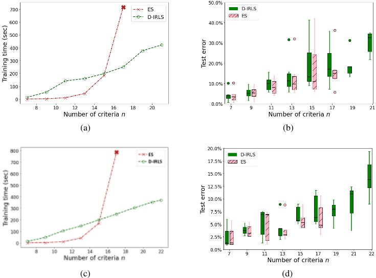
Training time and generalizing performance. In the first experiment, we generate 10 training/test sets and evaluate the average training time of both algorithms as well as the generalizing performances of the learned models (average preference inversion on a test set). In order to evaluate the scalability of our method we vary the number of criteria from n = 7 to n = 22. Figure 1 shows the results for the learning of the multilinear model (1a,1b) and for the Choquet integral in its conjunctive form (1c,1d). We observe that for both decision models ES does not provide any solution after n = 17.
| n | ˜ C(n) | C(n) | Time ESG | Time ESC |
| 6 | 3.2±6.4 | 192 | 0.6±0.2 | 0.6±0.1 |
| 9 | 2.4±7.2 | 2304 | 4.2±1.9 | 18.0±4.6 |
| 12 | 151.9±222.2 | 24576 | 61.0±30.4 | 1212.6±247.6 |
| 15 2777.6±4326.5 245760 3448.6±5613.1 - | ||||
However D-IRLS allows more than 4 millions of coefficients (n = 22) to be learned in less than 450 seconds. In contrast we observe that the generalizing performances of the learned decision models obtained with D-IRLS and ES are comparable. Since the number of training preference examples is constant, the test error globally increases with the number of criteria for both methods. Finally, we can notice that the test errors obtained for the learning of MLv are higher than the one obtained for the learning of Cv.
Enforcing monotonicity. In a second experiment, we assess the computational efficiency of the constraint generation algorithm used to guarantee monotonicity. We use the same experimental setting as above and let n vary from 6 to 15. We compare the exact solving of P under all monotonicity constraints (denoted ESC) with the exact solving of P with constraint generation (denoted ESG). Both are solved using LP. In Table 1 we compare C(n) the total number of monotonicity constraints in ESC, and ˜ C(n) the average number of constraints generated in ESG. We observe that ESC (including all contraints) is slower than ES and limited to n = 12. ESG performs significantly better (up to 15 criteria) due to the progressive introduction of monotonicity constraints. We observe that only a small fraction of the entire set of monotonicity constraints are inserted before reaching an optimal and fully monotonic capacity.
Comparison with k-additive models. The advantage of using sparse models with possible large interactions instead of k-additive models is illustrated in Table 2 where we compare our method (D-IRLS) to an exact solving of P with k-additivity constraints for k = 2 (2-add) and k = 3 (3add), still under the same experimental setting. The generalizing performance is significantly improved while computation times remain admissible (and even better for a large n).
| Test Error | Training time | |||||
|---|---|---|---|---|---|---|
| n | D-IRLS | 2-add | 3-add | D-IRLS | 2-add | 3-add |
| 8 | 0.04 | 0.10 | 0.06 | 28.22 | 1.33 | 1.40 |
| 12 | 0.04 | 0.17 | 0.23 | 122.53 | 20.96 | 21.34 |
| 16 | 0.06 | 0.22 | 0.49 | 187.79 | 345.13 | 346.78 |
Mixing different models of interactions. Preference learning produces an instance of model F(x) defined by Eq. 7. M¨obius coefficients mS are learned for any given monotonic function ϕS defining the nature of interaction terms.
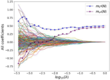
Several interaction functions may coexist in the same model with a possible benefit in terms of sparsity. As an illustration, we randomly draw preference examples (noised) based on the Hurwicz criterion: h(x) = 1 2 (mini∈N {xi} + maxi∈N {xi}). Although the min (resp. max) term admits a sparse representation in the conjunctive form (Eq. 5) of the Choquet integral (resp. disjunctive form, Eq. 6) this is not the case of h(x) that includes both terms. This suggests extending the model defined in Eq. 7 to include simultaneously several instances of ϕS (like min and max). If we write v = v∧ +v∨ with (v∧,v∨) two sub-normalized capacities, we have Cv(x) = Cv∧(x) + Cv∨(x). Then using the conjunctive form for Cv∧(x) and the disjunctive form for Cv∨(x) we obtain: Cv(x) = ∑S⊆N (mv∧ (S) mini∈S{xi}+m¯ v∨(S)maxi∈S{xi}). Then we compute a sparse representation of Cv possibly including both conjunctive and disjunctive terms by solving a variant of problem P using the double penalization term λ∧ ∑j>n |mv∧(j)| + λ∨ ∑j>n |m¯ v∨ (j)| under the normalization constraint ∑S⊆N (mv∧ (S) + m¯ v∨(S)) = 1. On Figure 2 we provide the regularization path obtained for increasing values of λ∧ = λ∨. As expected, a model including only two factors (min and max) is progressively emerging.
5 Conclusion
We have addressed the problem of preference learning with interacting criteria by considering a large class of capacitybased decision models including the multilinear utility and the Choquet integral, known for their expressiveness. We proposed a unified approach to learn the models of this class based on the search of sparse M¨obius representations of capacities, leading to simple models with sparse interaction patterns. This approach applies to instances possibly involving more than 20 criteria and allows the most significant interaction factors to be identified within millions of possibilities. This represents a significant improvement compared to previous approaches limited to a dozen of criteria. Moreover, the sparsity pattern is revealed from preference examples instead of resulting from a prior cardinality-based simplification of interactions, which greatly enhances the descriptive possibilities. The main directions to extend this work are 1) going further in scalability (a larger use of kernels is worth investigating) and 2) extending the approach to learn interaction functions ϕS from preference data (model selection problem).
Acknowledgments
This work is supported by the ANR project ANR-20-CE230018 THEMIS of the French National Research Agency.
@inproceedings{ijcai2023p421,
  title     = {Learning Preference Models with Sparse Interactions of Criteria},
  author    = {Herin, Margot and Perny, Patrice and Sokolovska, Nataliya},
  booktitle = {Proceedings of the Thirty-Second International Joint Conference on
               Artificial Intelligence, {IJCAI-23}},
  publisher = {International Joint Conferences on Artificial Intelligence Organization},
  editor    = {Edith Elkind},
  pages     = {3786--3794},
  year      = {2023},
  month     = {8},
  note      = {Main Track},
  doi       = {10.24963/ijcai.2023/421},
  url       = {https://doi.org/10.24963/ijcai.2023/421},
}
TY - CPAPER TI - Learning Preference Models with Sparse Interactions of Criteria AU - Herin, Margot AU - Perny, Patrice AU - Sokolovska, Nataliya T2 - Proceedings of the Thirty-Second International Joint Conference on Artificial Intelligence, IJCAI-23 PB - International Joint Conferences on Artificial Intelligence Organization PY - 2023 SP - 3786 EP - 3794 DO - 10.24963/ijcai.2023/421 UR - https://doi.org/10.24963/ijcai.2023/421 ER -Copied
Machine-readable versions of this paper, for tools and AI agents:





