
CRAFT: Time Series Forecasting with Cross-Future Behavior Awareness
Proceedings of the Thirty-Fourth International Joint Conference on Artificial Intelligence. Main Track. Pages 7056-7064.
https://doi.org/10.24963/ijcai.2025/785
Keywords
- Machine Learning: ML: Time series and data streams
- Machine Learning: ML: Applications
Abstract
The past decades witness the significant advancements in time series forecasting (TSF) across various real-world domains, including e-commerce and disease spread prediction. However, TSF is usually constrained by the uncertainty dilemma of predicting future data with limited past observations. To settle this question, we explore the use of Cross-Future Behavior (CFB) in TSF, which occurs before the current time but takes effect in the future. We leverage CFB features and propose the CRoss-Future Behavior Awareness based Time Series Forecasting method (CRAFT). The core idea of CRAFT is to utilize the trend of cross-future behavior to mine the trend of time series data to be predicted. Specifically, to settle the sparse and partial flaws of cross-future behavior, CRAFT employs the Koopman Predictor Module to extract the key trend and the Internal Trend Mining Module to supplement the unknown area of the cross-future behavior matrix. Then, we introduce the External Trend Guide Module with a hierarchical structure to acquire more representative trends from higher levels. Finally, we apply the demand-constrained loss to calibrate the distribution deviation of prediction results. We conduct experiments on real-world dataset. Experiments on both offline large-scale dataset and online A/B test demonstrate the effectiveness of CRAFT. Our dataset and code are available at https://github.com/CRAFTinTSF/CRAFT.
- [Avati et al., 2020] Anand Avati, Tony Duan, Sharon Zhou, Kenneth Jung, Nigam H Shah, and Andrew Y Ng. Count- down regression: sharp and calibrated survival predictions. In Uncertainty in Artificial Intelligence, pages 145-155.
- PMLR, 2020.
- [Bai et al., 1803] Shaojie Bai, J Zico Kolter, and Vladlen Koltun. An empirical evaluation of generic convolutional and recurrent networks for sequence modeling. arxiv 2018. arXiv preprint arXiv:1803.01271, 2(1803):8, 1803.
- [Chen et al., 2020] Yitian Chen, Yanfei Kang, Yixiong Chen, and Zizhuo Wang. Probabilistic forecasting with temporal convolutional neural network. Neurocomputing, 399:491-501, 2020.
- [Gao et al., 2022] Chengliang Gao, Fan Zhang, Yue Zhou, Ronggen Feng, Qiang Ru, Kaigui Bian, Renqing He, and Zhizhao Sun. Applying deep learning based probabilistic forecasting to food preparation time for on-demand deliv- ery service. In Proceedings of the 28th ACM SIGKDD Conference on Knowledge Discovery and Data Mining, pages 2924-2934, 2022.
- [Glorot and Bengio, 2010] Xavier Glorot and Yoshua Ben- gio. Understanding the difficulty of training deep feedfor- ward neural networks. In Proceedings of the thirteenth in- ternational conference on artificial intelligence and statis- tics, pages 249-256. JMLR Workshop and Conference Proceedings, 2010.
- [Hu et al., 2024] Xuanming Hu, Wei Fan, Haifeng Chen, Pengyang Wang, and Yanjie Fu. Reconstructing missing variables for multivariate time series forecasting via con- ditional generative flows. In Proceedings of the 33rd In- ternational Joint Conference on Artificial Intelligence (IJ- CAI), Jeju, Korea, 2024. IJCAI
- [Koopman, 1931] Bernard O Koopman. Hamiltonian sys- tems and transformation in hilbert space. Proceedings of the National Academy of Sciences, 17(5):315-318, 1931.
- [Li et al., 2024] Yuxin Li, Wenchao Chen, Xinyue Hu, Bo Chen, Mingyuan Zhou, et al. Transformer-modulated diffusion models for probabilistic multivariate time series forecasting. In The Twelfth International Conference on Learning Representations, 2024.
- [Lim et al., 2021] Bryan Lim, Sercan Ö Arık, Nicolas Lo- eff, and Tomas Pfister. Temporal fusion transformers for interpretable multi-horizon time series forecasting. Inter- national Journal of Forecasting, 37(4):1748-1764, 2021.
- [Liu et al., 2020] Fan Liu, Xingshe Zhou, Jinli Cao, Zhu Wang, Tianben Wang, Hua Wang, and Yanchun Zhang. Anomaly detection in quasi-periodic time series based on automatic data segmentation and attentional lstm-cnn. IEEE Transactions on Knowledge and Data Engineering, 34(6):2626-2640, 2020.
- [Liu et al., 2021] Shizhan Liu, Hang Yu, Cong Liao, Jian- guo Li, Weiyao Lin, Alex X Liu, and Schahram Dust- dar. Pyraformer: Low-complexity pyramidal attention for long-range time series modeling and forecasting. In Inter- national conference on learning representations, 2021.
- [Liu et al., 2024a] Yong Liu, Tengge Hu, Haoran Zhang, Haixu Wu, Shiyu Wang, Lintao Ma, and Mingsheng Long. itransformer: Inverted transformers are effective for time series forecasting. In The Twelfth International Confer- ence on Learning Representations, 2024.
- [Liu et al., 2024b] Yong Liu, Chenyu Li, Jianmin Wang, and Mingsheng Long. Koopa: Learning non-stationary time series dynamics with koopman predictors. Advances in Neural Information Processing Systems, 36, 2024.
- [Lu et al., 2022] Yucheng Lu, Qiang Ji, Liang Wang, Tian- shu Wu, Hongbo Deng, Jian Xu, and Bo Zheng. Star- dom: semantic aware deep hierarchical forecasting model for search traffic prediction. In Proceedings of the 31st ACM International Conference On Information & Knowl- edge Management, pages 3352-3360, 2022.
- [Mendis et al., 2024] Kasun Mendis, Manjusri Wickramas- inghe, and Pasindu Marasinghe. Multivariate time series forecasting: A review. In Proceedings of the 2024 2nd Asia Conference on Computer Vision, Image Processing and Pattern Recognition, pages 1-9, 2024.
- [Mossop and Rahman, 2023] Brandon Mossop and Quazi Abidur Rahman. Infectious disease forecast- ing using multivariate incomplete time-series: A hybrid architecture with stacked dilated causal convolutions. In 2023 IEEE International Conference on Bioinformatics and Biomedicine (BIBM), pages 4220-4227. IEEE, 2023.
- [Nie et al., 2024] Yuqi Nie, Nam H Nguyen, Phanwadee Sinthong, and Jayant Kalagnanam. A time series is worth 64 words: Long-term forecasting with transformers. In The Eleventh International Conference on Learning Rep- resentations, 2024.
- [Oord et al., 2016] Aaron van den Oord, Sander Diele- man, Heiga Zen, Karen Simonyan, Oriol Vinyals, Alex Graves, Nal Kalchbrenner, Andrew Senior, and Koray Kavukcuoglu. Wavenet: A generative model for raw au- dio. arXiv preprint arXiv:1609.03499, 2016.
- [Rasul et al., 2024] Kashif Rasul, Andrew Bennett, Pablo Vicente, Umang Gupta, Hena Ghonia, Anderson Schnei- der, and Yuriy Nevmyvaka. Vq-tr: Vector quantized at- tention for time series forecasting. In The Twelfth Interna- tional Conference on Learning Representations, 2024.
- [Salinas et al., 2020] David Salinas, Valentin Flunkert, Jan Gasthaus, and Tim Januschowski. Deepar: Probabilistic forecasting with autoregressive recurrent networks. Inter- national Journal of Forecasting, 36(3):1181-1191, 2020.
- [Shetty and Ismail, 2023] Dileep Kumar Shetty and B Is- mail. Forecasting stock prices using hybrid non-stationary time series model with ernn. Communications in Statistics-Simulation and Computation, 52(3):1026-1040, 2023.
- [Wang et al., 2019] Yuyang Wang, Alex Smola, Danielle Maddix, Jan Gasthaus, Dean Foster, and Tim Januschowski. Deep factors for forecasting. In In- ternational conference on machine learning, pages 6607-6617. PMLR, 2019.
- [Wang et al., 2024] Xue Wang, Tian Zhou, Qingsong Wen, Jinyang Gao, Bolin Ding, and Rong Jin. Card: Channel aligned robust blend transformer for time series forecast- ing. In The Twelfth International Conference on Learning Representations, 2024.
- [Wen et al., 2017] Ruofeng Wen, Kari Torkkola, Balakrish- nan Narayanaswamy, and Dhruv Madeka. A multi- horizon quantile recurrent forecaster. arXiv preprint arXiv:1711.11053, 2017.
- [Wen et al., 2023] Qingsong Wen, Tian Zhou, Chaoli Zhang, Weiqi Chen, Ziqing Ma, Junchi Yan, and Liang Sun. Transformers in time series: a survey. In Proceedings of the Thirty-Second International Joint Conference on Arti- ficial Intelligence, pages 6778-6786, 2023. IJCAI
- [Wu et al., 2021] Haixu Wu, Jiehui Xu, Jianmin Wang, and Mingsheng Long. Autoformer: Decomposition transform- ers with auto-correlation for long-term series forecast- ing. Advances in neural information processing systems, 34:22419-22430, 2021.
- [Yang et al., 2024] Yingnan Yang, Qingling Zhu, and Jiany- ong Chen. Vcformer: Variable correlation transformer with inherent lagged correlation for multivariate time se- ries forecasting. Proceedings of the 33rd International Joint Conference on Artificial Intelligence (IJCAI), Jeju, Korea, 2024. IJCAI
- [Yin et al., 2022] Changchang Yin, Sayoko E Moroi, and Ping Zhang. Predicting age-related macular degenera- tion progression with contrastive attention and time-aware lstm. In Proceedings of the 28th ACM SIGKDD Confer- ence on Knowledge Discovery and Data Mining, pages 4402-4412, 2022.
- [Zeng et al., 2023] Ailing Zeng, Muxi Chen, Lei Zhang, and Qiang Xu. Are transformers effective for time series fore- casting? In Proceedings of the AAAI conference on artifi- cial intelligence, volume 37, pages 11121-11128, 2023.
- [Zhang et al., 2025] Yingwei Zhang, Ke Bu, Zhuoran Zhuang, Tao Xie, Yao Yu, Dong Li, Yang Guo, and De- tao Lv. Craft: Time series forecasting with cross-future behavior awareness, 2025.
- [Zhao and Shen, 2024] Lifan Zhao and Yanyan Shen. Re- thinking channel dependence for multivariate time series forecasting: Learning from leading indicators. In The Twelfth International Conference on Learning Represen- tations, 2024.
- [Zhou et al., 2021] Haoyi Zhou, Shanghang Zhang, Jieqi Peng, Shuai Zhang, Jianxin Li, Hui Xiong, and Wan- cai Zhang. Informer: Beyond efficient transformer for long sequence time-series forecasting. In Proceedings of the AAAI conference on artificial intelligence, volume 35, pages 11106-11115, 2021.
- [Zhou et al., 2022] Tian Zhou, Ziqing Ma, Qingsong Wen, Xue Wang, Liang Sun, and Rong Jin. Fedformer: Fre- quency enhanced decomposed transformer for long-term series forecasting. In International conference on machine learning, pages 27268-27286. PMLR, 2022.
- [Zhu et al., 2023] Ruitao Zhu, Detao Lv, Yao Yu, Ruihao Zhu, Zhenzhe Zheng, Ke Bu, Quan Lu, and Fan Wu. Linet: A location and intention-aware neural network for hotel group recommendation. In Proceedings of the ACM Web Conference 2023, pages 779-789, 2023.
- [Zonghan et al., 2019] Wu Zonghan, Pan Shirui, Long Guodong, Jiang Jing, and Zhang Chengqi. Graph wavenet for deep spatial-temporal graph modeling. In Proceed- ings of the Twenty-Eighth International Joint Conference on Artificial Intelligence, IJCAI 2019, Macao, China, Au- gust 10-16, 2019, pages 1907-1913, 2019. IJCAI
References were extracted automatically from the PDF and may contain errors.
Full text extracted automatically from the PDF; figures, tables and equations may differ. The PDF is the version of record.
1 Introduction
Time series forecasting (TSF) is the crucial infrastructure of various real-world domains, including e-commerce [Wen et al., 2017], traffic [Hu et al., 2024], disease spread prediction [Mossop and Rahman, 2023], and stock price prediction [Shetty and Ismail, 2023].
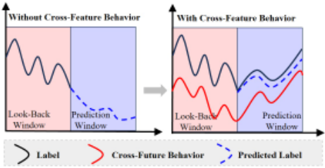
However, accurate TSF is a challenging task given the need to model complex, non-linear temporal patterns over long periods of time [Rasul et al., 2024]. To this end, researchers explore various backbone networks such as convolutional neural networks (CNNs) [Chen et al., 2020], recurrent neural networks (RNNs) [Yin et al., 2022], and Transformer [Zhou et al., 2021]. Additionally, they work on incorporating richer features into TSF and study issues related to multivariate TSF [Zhao and Shen, 2024; Li et al., 2024] and feature decomposition [Zeng et al., 2023; Liu et al., 2024b]. With the advancement of sensing technology, such as Internet data in e-commerce and population mobility information in disease spread prediction, various priori information for TSF can be recorded. In this paper, we defined these priori information as Cross-Future Behavior (CFB): features that occur before the current time but take effect in the future. CFB positively affects TSF. As shown in Figure 1, if only relying on the trend of the label, the future trend may be predicted as a downward trend. With the guidance of CFB, the prediction result will be more precise.
In fact, existing work is also attempting to introduce more features into TSF. [Zeng et al., 2023] attempts to extract more information from the acquired data and decomposes the time series into trend and remainder parts. [Wen et al., 2017] classifies covariate features in TSF into dynamic historical, known future, and static variables. CFB, we proposed in this paper, can be treated as the known future variable and has many excellent properties. CFB contains true information related to future events. The future trend of the prediction target, even the abnormal trend caused by sudden events, can be reflected in the trend of CFB. However, as the existing TSF models primarily focus on exploring the correlation between the historical series and future trends [Chen et al., 2020; Yin et al., 2022; Zhou et al., 2021], it is difficult to achieve TSF that integrates CFB through existing models. Taking the e-commerce scenario as an example, CFB-based TSF faces two main challenges. 1) CFB is sparse and partial. Consumers can book items at any time, causing CFB to remain fully observed until the last minute. Thus, if CFB is simply incorporated into the model, the prediction model may be unable to apply CFB features correctly and even make incorrect predictions due to CFB. 2) The trend of CFB is unobvious. Compared with the sales trend in a business district, the sales trend in an individual hotel is unobvious. CFB has the same nature, and the trend in an individual hotel is much unobvious compared with that in a high-level business district. Consequently, devising a method to utilize the sales trend in high level to inform the auxiliary forecast for an individual hotel presents another significant challenge.
Therefore, jointly considering the above challenges, we propose CRAFT, a Cross-Future Behavior Awareness based Time Series Forecasting method, for the first time to utilize Cross-Future Behavior to realize time series forecasting. The core idea of CRAFT, as shown in Figure 1, is to utilize the trend of CFB to mine the trend of time series data to be predicted. CRAFT is composed of three main parts: the Koopman Predictor Module (KPM), the Internal Trend Mining Module (ITM), and the External Trend Guide Module (ETG). KPM can extract the key trends of the label and CFB, predicting the label in the prediction window. ITM supplements the unknown area of CFB, making the final prediction of the label in the prediction window. ETG, with a hierarchical structure, can acquire more representative trends from higher levels. Finally, we apply the demand-constrained loss to calibrate the distribution deviation of prediction results. We conduct experiments on real-world dataset. Experiments on both offline large-scale dataset and online A/B test demonstrate the effectiveness of CRAFT. We summarize the main contributions of this paper as follows:
- We define CFB and apply CFB to TSF for the first time. CFB is a feature discovered from our extensive real case studies and has superior characteristics: the trend of CFB can reflect the prediction target and even the abnormal trend of the target.
- We propose a novel framework, namely CRAFT, to realize CFB-based time series forecasting. CRAFT can utilize the trend of CFB to mine the trend of prediction targets. CRAFT is composed of three main modules, including KPM, ITM, and ETG. KPM and ITM can address the sparse and partial flaws of CFB, and ETG can address the unobvious trend flaws of CFB.
- Extensive offline experiments on the real-world dataset and online A/B tests show the superiority of CRAFT towards SOTA baselines. CRAFT improves application performance significantly, with an improvement rate of 41.35% on the IWR metric. Currently, CRAFT has been successfully deployed on the reality application.
2 RelatedWork
Backbone for time series forecasting. Recently, Transformer has reshaped the landscape of TSF across numerous fields [Wen et al., 2023]. PatchTST [Nie et al., 2024] designs a channel-independent Transformer for time series forecasting. To address the channel-independent limitations of Transformer, CARD [Wang et al., 2024] proposes a channel-aligned attention structure that can acquire both temporal correlations and dynamical dependence among multiple variables over time. Informer [Zhou et al., 2021] extends Transformer using ProbSparse based on KL divergence to solve Long Sequence time series forecasting. TFT [Lim et al., 2021] introduces a novel attention-based architecture that combines high-performance multi-horizon forecasting with interpretable insights into temporal dynamics. Autoformer [Wu et al., 2021] proposes a Decomposition Architecture and Auto-Correlation Mechanism based on stochastic process theory to realize the series-wise connection and break the bottleneck of information utilization. Pyraformer [Liu et al., 2021] proposes a new Transformer based on a pyramidal attention module to simultaneously capture temporal dependencies of different ranges in a compact multi-resolution fashion. Besides Transformer, a variety of other network architectures are widely investigated. CNNs-based time series forecasting models such as WaveNet [Oord et al., 2016], TCN [Bai et al., 1803], and DeepTCN [Chen et al., 2020] use causal convolution to learn sequences and use dilated convolution and residual block to memorize historical patterns. Graph WaveNet [Zonghan et al., 2019] enhances the WaveNet framework by using an adaptive and learnable adjacency matrix to automatically infer graph structures, enabling the prediction of spatiotemporal sequences. Moreover, due to the sequential nature of time series data, RNNs-based time series forecasting is particularly widely suited, mainly modeling the temporal dependence of time series [Salinas et al., 2020; Wang et al., 2019; Liu et al., 2020].
Multivariate time series forecasting. Multivariate TSF utilizes multiple time-dependent variables to realize prediction. Compared with univariate TSF, multivariate TSF can understand the interactions between different components of a complex system better, which is crucial for strategy formulation and decision-making [Mendis et al., 2024]. There are two commonly used strategies in multivariate TSF, i.e., the channel-dependent (CD) and channel-independent (CI) methods. CI method only models cross-time dependence, and the CD method models both cross-time dependence and crossvariate dependence [Zhao and Shen, 2024; Yang et al., 2024]. While the CI method is characterized by simplicity and low risk of overfitting, the CD method has inevitably become the mainstream of research. Recently, [Zhao and Shen, 2024] utilizes the channel dependence between variates and proposes a plug-and-play method named LIFT, which exploits the leadlag relationship between variates by estimating leading indicators and leading steps, refreshing multivariate TSF's performance.
Feature decomposition in time series forecasting. Different from multivariate TSF utilizing multiple variates and the dependence between variates to realize prediction, feature decomposition in TSF does not introduce new variates. The core idea of feature decomposition is to extract as much information as possible from existing variates. Dlinear [Zeng et al., 2023] decomposes time series into trend series and remainder series and uses two single-layer linear networks to model them, bringing performance improvements. Koopa [Liu et al., 2024b] solves non-stationary time series prediction problems from the perspective of modern dynamics Koopman theory.
3 Preliminaries
Time series forecasting (TSF) with Cross-Future Behavior (CFB) can be defined as Yt+1:t+P = H(Yt-L+1:t,XT,CT). Yt-L+1:t ∈ RL and Yt+1:t+P ∈ RP are time series data (i.e., label) at the L-length look-back window and P -length prediction window at time t respectively. XT is covariate features, CT is the CFB feature and H is the prediction function to be learned. The covariate features [Wen et al., 2017] XT contains three categories: 1) historical features like month-on-month sales features, etc; 2) known future features like holidays, weekends, etc; 3) static features like hotel brands, business districts, etc. CT = {Ct-L+1:t, Ct+1:t+P }, where Ct-L+1:t is CFB in the look-back window and Ct+1:t+P is CFB in the prediction window. It is worth noting that Ct+1:t+P in the prediction window is partial as this is a not fully observable variate. Consumers can book items in the prediction window at any time until the last minute. More detailed introduction to CFB feature Ct refers to Appendix A in our full paper [Zhang et al., 2025].
In the following section, we omit the subscripts of some symbols for simplicity. Specifically, we denote time series at the look-back windowYt-L+1:t as YL, time series at the prediction window Yt+1:t+P as YP , CFB feature in lookback window Ct-L+1:t as CL, CFB feature in prediction window Ct+1:t+P as CP . In addition, as CP is partial observed, we define a new notion CTP to indicate the ground truth of CFB in prediction window.
4 Methodology
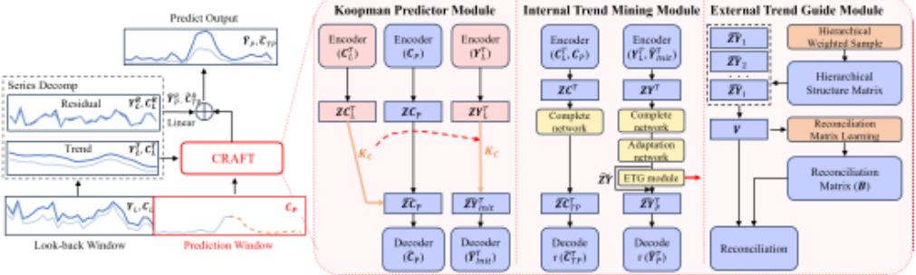
Figure 2 depicts the overview of the proposed CRAFT method. CRAFT uses DLinear [Zeng et al., 2023] to decompose the time series data YL,CL in the look-back window into the trend YTL , CTL and residual YR L = YL - YTL , CRL = CL - CTL components. The moving average kernel with a certain kernel size is used in the decomposition process. CRAFT's core idea lies in how to use the trend of partial CFB to mine the trend of label. We prove the consistency between partial CFB, CFB, and label theoretically in Appendix D.1 and D.2 in our full paper [Zhang et al., 2025]. CRAFT is composed of three submodules: Koopman Predictor Module (KPM), Internal Trend Mining Module (ITM), and External Trend Guide Module (ETG). KPM employs the Koopman operator to linearly map the CFB features from the look-back window to the prediction window, after projecting the raw data into the mapping space. Subsequently, it supervises the initialization of the label sequence within the prediction window. ITM completes linear mapping between the look-back window and prediction window and adopts an adaptation operator to instruct the evolution of the time series of the label sequentially. Due to higher-level temporal sequences having lower noise and stronger regularity compared to lowerlevel temporal sequences, ETG module makes forecast results more robust by structuring the reconciliation matrix and calibrating the predicted outcomes of root nodes. To avoid computational problems caused by excessively large hierarchical matrices, the concept of hierarchical sampling is introduced.
4.1 Koopman Predictor Module
KPM module aims to transfer the future trend information from CFB feature CT = {CL,CP} to labels YP . The simplified framework of KPM is shown in Figure 2 and the specific framework refers to Appendix C.1 in our full paper [Zhang et al., 2025]. KPM employs an encoder-decoder framework with the input of CFB CL and label YL in the look-back window and output of partial CFB CP in the prediction window. Concretely, we first construct an encoder RL ↦→ RD as a data-driven measurement function. The encoder module is Multi Layer Perception (MLP) [Zhu et al., 2023] and it can also be replaced to other structure: ZCTL = Encoder(CTL ),ZCP = Encoder(CP ),ZYTL = Encoder(YTL ), where ZCTL ,ZCP ,ZYTL are the embeddings of the trend of CFB in the look-back window, CFB in the prediction window, and the trend of labels in the look-back window. In particular, the encoder is shared for ZCTL , ZCP , ZYTL . Secondly, based on the Koopman Theory [Koopman, 1931], we use finite linear matrix KC to approach infinite koopman matrix K to simulate the evolution process between time periods, that is:
where KC ∈ RD×D is the Koopman matrix for CFB, which contains the future sales trend information. Its value can be approximated by ridge regression as:
Then, we use KC to convert the future trend information from CFB embedding to label embedding:
Finally, we construct a decoder RD ↦→ RP to obtain the preliminary prediction result of label. Same as encoder, decoder can adopt various model structures, and this paper uses the MLP layer [Zhu et al., 2023]. In particular, the decoder is shared for ˆCP , ˆYT Init : ˆCP = Decoder( ˆ ZCP ), ˆYT Init = Decoder( ˆ ZYTInit ). Specifically, to ensure that KC is meaningful, we construct a recovery loss Lbe k to constrain the decoder to restore the original data based on the embedding output by the encoder, so that the embedded latent variable enables to obtain the potential attributes from raw data and preserve the original information as much as possible. Lbe k is designed based on the MSE loss:
we choose CP to calculate loss because we emphasize more on tendency characterization at the prediction window. It should be noted that we only focus on the known parts, i.e., j ≤ i, and the loss of the masked data will not be calculated.
4.2 Internal TrendMiningModule
ITM module aims to complete the CFB feature. After KPM, we attained preliminary insufficient prediction ˆYT Init . In the ITM module, we first adopt a complete network to patch the mapping of CFB from the look-back window to the prediction window and then employ an adaptation network to fulfill the adaptive migration of data distribution from CFB to the label. The simplified framework is in Figure 2 and the specific framework is in Appendix C.2 in our full paper [Zhang et al., 2025]. We utilize another pair of encoder RL+P ↦→ RD and decoder RD ↦→ RL+P to learn the common embedding for entire known information. Unlike KPM, ITM takes all known information as input, i.e., data in the train and prediction window. Regarding the label, we pad preliminary predicted values ˆYT Init at the prediction window: ZCT = Encoder(concat(CTL , CP )), ZYT = Encoder(concat(YTL , ˆYT Init )). To settle the forecast window puzzle, we use the complete network to extend known curves into unknown regions, which is designed as a linear network:
Additionally, despite there being a certain correlation between CFB and label, their distributions are not entirely identical. Based on this fact, we employ an adaptation network to adjust the label adaptively, with the ETG module (4.3) following closely behind. Since both the complete network and adaptation network operate on the hidden variable ZYT based on the original attributes of labels, we merge them into the ITM module to distinguish it from the ETG module. After traversing from the ITM & ETG module, we acquire the desired latent variable ˆ ZYTP :
Finally, the latent vector ˆ ZCTTP and ˆ ZYTP are converted into target predicted values with decoder: ˆCTTP = Decoder( ˆ ZCTTP ), ˆ Y T P =Decoder( ˆ ZYTP ).
The final result is calculated by adding these two values with the reminder predicted values (acquired with the linear mapping of YR L ,CRL in Figure 2, ˆCRTP = Linear(CRL ), ˆ Y R P = Linear(YR L )):
To ensure the effectiveness of complete network, we introduce the prediction bias loss Lbe y:
4.3 External Trend Guide Module
ETG module is designed to settle the trend unobvious challenge, which uses aggregated spatial dimension to improve prediction results. Aggregated spatial dimension has stronger regularity, less noise, and is easier to estimate. Table 1 shows that the sample size of the hotel is approximately 400k, which is too extensive for direct model train. Therefore, referring to [Lu et al., 2022], we introduced a hierarchical sampling strategy to construct samples. This strategy assumes the global reconciliation matrix P is sparse, indicating that only child nodes belonging to the same parent node have calibration relationships with each other. This assumption aligns well with the geographic attributes of hotels. We aggregate hotels into business districts based on their geographic location and then to higher levels of urban granularity. First, we randomly pick a business district. Then, we sample m hotels from this district, with the likelihood of selection increasing with each hotel's historical label value. These m hotels' labels are combined to create a virtual parent node. Together, the m + 1 nodes form a sampled hierarchy that serves as model input. This hierarchical sampling maintains the sum constraint through virtual parent nodes, and label weighted sampling aligns the virtual sequence more with the real parent sequence. Moreover, these strategies reduce the reconciliation matrix's parameter count from O(n2 ) to O(mn), significantly easing the model's computational load.
The framework of ETG is detailed in Figure 2 and Appendix C.3 in our full paper [Zhang et al., 2025]. The input of ETG is ˜ ZY (Eq. (6)). zi/j/k = ˜ ZY[i/j/k] are the elements of ˜ ZY. According to the hierarchical sampling, we can adjust its shape from [Bt, · · · ] to [g,m, · · · ], where Bt = g×m, indicating the number of original nodes, the number of nodes in high-level and in low-level. All subsequent actions are operated within the virtual hierarchical group. We obtain the key and query to calculate the reconciliation matrix B between nodes in the same hierarchical structure, where B(i, j) indicates the reconciliation relationship between the ith and jth nodes in the hierarchical structure:
where Wq ∈ Rd×d ,Wk ∈ Rd×d are the query and key parameter of model, Mi is the set of nodes in the current hierarchy of i. Then, we use the reconciliation matrix B to calibrate each sequence:
whereWv ∈ Rd×d is the model's value parameter. Given the lower noise and greater regularity of parent nodes compared to child nodes, we refrain from applying representation calibration to parent nodes using masking techniques, aligning with the reconciliation process. During the model training process, we introduce reconciliation loss to implement hierarchical constraints:
where ˆYP [iH ] is the estimated result of parent node. Lrecon indicates the difference between the direct estimation of the parent node and sum of underlying estimation results, ensuring the sum of the calibrated estimated results of the underlying nodes approach parent node's estimated results.
4.4 Algorithm Inference
To fully utilize demand information related to cross-future behavior, we constructed the demand-constrained loss. In practice, we have found that there are invisible boundaries on the amount of user demand. Inspired by [Avati et al., 2020; Gao et al., 2022], we are conscious that the boundary is informative for the model. Thus, we construct upper and lower limits based on the demand in transaction scenarios and design a demand-constrained loss to digest this boundary information. The principle is shown in Figure 3. From the perspective of likelihood estimation, we make assumptions about the distribution of labels when using the common MAE or MSE as a loss function. Taking the MSE loss function used in this paper as an example, the MSE loss function is based on the assumption that the predicted target follows a Gaussian distribution, and what our model infers is the mean of the Gaussian distribution. The actual observation may not necessarily be the mean of true Gaussian distribution. With the assistance of upper and lower limits, we can support the model hover the true distribution.
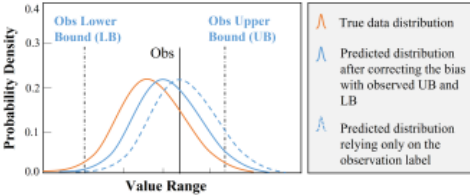
In the check-in scenario of the hotel, we regard the truth value as label y (i.e., Y) and regard the value for the day of reservation as the lower demand bounds yl, excluding entire CFB actions. We also consider the page view of the order page as the upper bound yu, including the unconverted potential user data. The demand-constrained loss is as follows:
where β is hyperparameter. We define the main loss as Ly, indicating the forecast bias of YP :
where YL P is the lower bound matrix, and YU P is the upper bound matrix. Through the aforementioned submodules, CRAFT enables the future trend of cross-future behavior to approach consummation and migrate it to the tendency cognition of label, aggregating to higher-level label to perceive more distinct and precise inclination subsequently. During the process, we obtain ˆCP which is transferred from encoder to decoder to constrain the representation of koopman embedding, the intact matrix expression of prediction window of cross-future behavior ˆCTP , and ultimate desired prediction results ˆYP . To achieve better model outcome, the loss of CRAFT consists of four parts, where αn, n ∈ 1, 2, 3 are hyper parameters used to balance multiple losses:
Lbe k, Lbe y, Lrecon, Ly are shown in Eq. (4), Eq. (8), Eq. (11), and Eq. (12) which corresponding to the recovery loss of ˆCP in the KPMmodule, the prediction error of ˆCTP in the ITMmodule, the reconstruction drift of ˆYP at the ETG module and the forecast deviation of label ˆYP respectively.
5 Experiments
5.1 Experimental Settings
Dataset
We conduct offline experiments on real-world dataset collected in May 2023 at Fliggy. To reflect the model effects on different data distributions objectively, the prediction window we cover to verify the model's effectiveness contains both holidays and daily events. In addition, we set different forecast lengths K ∈ {7, 14, 30}, corresponding to look-back lengths T ∈ {30, 90, 180}. The dataset statistics are shown in Table 1. The hotels we use for verification are located in over 400 cities, covering more than 5000 business districts. The total sample size is around 400k.
| Hierarchy | # of city | # of business | # of hotel |
| Volume | 0.4k | 5k | 400k |
Baseline Methods and Evaluation Metrics
The baseline methods for comparison include MQRNN [Wen et al., 2017], Informer [Zhou et al., 2021], DLinear [Zeng et al., 2023], Koopa [Liu et al., 2024b], TFT [Lim et al., 2021], Autoformer [Wu et al., 2021], Fedformer [Zhou et al., 2022] and iTransformer [Liu et al., 2024a].
Weighted Mean Absolute Percentage Error (wMAPE) is adopted to measure the models' performance in offline experiments:
where y denotes the ground truth and ˆ y denotes the predicted value. In hotel booking situations, the data distribution is a significant imbalance, adopting wMAPE as a performance metric can effectively alleviate zero values issues. In addition, wMAPE allows assigning different weights to different ground truth, thus increasing the evaluation robustness. In addition, MAE and RMSE, two widely used metrics in time series forecasting, are adopted to evaluate the models' performance.
Implementation
All experiments are implemented with Python 3.8.5 and Pytorch 1.12.1 We conduct them on the cloud servers with two NVIDIA Tesla T4 GPUs with 16GB VRAM each. We initialize the network parameters with Xavier Initialization [Glorot and Bengio, 2010]. Each parameter is sampled from N(0, µ2 ), where µ = -√2/(nin + nout). nin, nout denote the number of input and output neurons, respectively. In actuality, the λ of ridge regression for solving the koopman matrix in the ITMmodule is 0.1, the number of child nodes m at the virtual hierarchy is set as 15 during hierarchical sampling. In addition, we train all models by setting the mini-batch size to 256 and using the Adam optimizer with a learning rate of 0.001. Except for MQRNN with the quantile loss at 0.5, all other models choose MSE as the training loss. The number of training epochs is 2 on the dataset, and the value of each experimental result is the average of 5 repeated tests.
5.2 Offline Experiments
Comparison with Baselines
The comparative results are shown in Table 2. For fairness, we compared both the original baseline methods and the improved versions with CFB. CRAFT achieves the best performance, significantly outperforming the other baselines. We obtain the following observations from Table 2:
| Model | Length P | Only label | With CFB as covariate | ||||
|---|---|---|---|---|---|---|---|
| MAE | RMSE | wMAPE | MAE | RMSE | wMAPE | ||
| 7 days | 0.9319 | 2.9374 | 0.7030 | 0.9631 | 2.9132 | 0.7265 | |
| Autoformer 14 days | 1.0017 | 2.3737 | 0.9830 | 0.9799 | 2.3566 | 0.9624 | |
| 30 days | 0.9658 | 2.2737 | 0.9910 | 1.2101 | 2.7625 | 1.2414 | |
| 7 days | 0.9280 | 2.9147 | 0.7000 | 0.9191 | 2.9100 | 0.6933 | |
| Fedformer 14 days | 0.8744 | 2.3333 | 0.8605 | 0.9071 | 2.4167 | 0.8923 | |
| 30 days | 0.9109 | 2.1718 | 0.9347 | 1.6507 | 4.7499 | 1.6933 | |
| 7 days | 0.9584 | 2.9184 | 0.7195 | 0.9535 | 2.9043 | 0.7215 | |
| TFT 14 days | 0.8643 | 2.2745 | 0.8535 | 0.8524 | 2.2730 | 0.8468 | |
| 30 days | 0.8294 | 2.3346 | 0.8494 | 0.8301 | 2.2945 | 0.8693 | |
| 7 days | 0.9825 | 2.9539 | 0.7412 | 0.9822 | 2.9566 | 0.7410 | |
| DLinear 14 days | 0.8555 | 2.3279 | 0.8418 | 0.8571 | 2.3572 | 0.8427 | |
| 30 days | 0.8125 | 1.9499 | 0.8337 | 0.8089 | 1.9634 | 0.8298 | |
| 7 days | 0.9731 | 2.9251 | 0.7341 | 0.9365 | 2.9169 | 0.7065 | |
| Informer 14 days | 0.8034 | 2.2653 | 0.7906 | 0.8203 | 2.2969 | 0.8065 | |
| 30 days | 0.7699 | 1.9618 | 0.7899 | 0.8063 | 1.9844 | 0.8271 | |
| 7 days | 0.9057 | 2.9261 | 0.6832 | 0.9096 | 2.9086 | 0.6862 | |
| iTransformer 14 days | 0.7755 | 2.2896 | 0.7632 | 0.7891 | 2.3134 | 0.7758 | |
| 30 days | 0.8062 | 2.0475 | 0.7694 | 0.7720 0.9064 | 2.0144 3.0185 | 0.7364 | |
| 7 days | 3.0013 | 0.6895 | 0.6830 | ||||
| MQ-RNN 14 days | 0.9007 0.7403 | 2.5217 | 0.7478 | 0.7415 | 2.4554 | 0.7381 | |
| 30 days | 0.6958 | 2.1756 | 0.7142 | 0.7029 | 2.2161 | 0.7215 | |
| 7 days | 0.9024 | 2.9047 | 0.6943 | 0.8927 | 2.8948 | 0.6818 | |
| Koopa 14 days | 0.7440 | 2.3485 | 0.7326 | 0.7475 | 2.4327 | 0.7350 | |
| 30 days | 0.7045 | 2.1943 | 0.7276 | 0.6984 | 2.3456 | 0.7176 | |
| 7 days | 0.8480 | 2.8654 | 0.6706 | ||||
| CRAFT 14 days | 0.7237 | 2.2696 | 0.7121 | ||||
| 30 days | 0.6895 | 2.0121 | 0.7078 | ||||
- Compared to the original model, directly integrating CFB into the existing framework does not yield significant performance enhancements. In some cases, it even leads to performance degradation. The experimental results confirm that, despite its indispensable role, effectively applying CFB presents considerable challenges.
- Compared with the optimal baseline, CRAFT improves by at least {0.0447, 0.0166, 0.0063} and {0.0112, 0.0205, 0.0064} in MAE and wMAPE metrics in the prediction window of {7, 14, 30}. In RMSE metric, CRAFT ranks the best and the second best when the length of prediction window is 7 and 14. To sum up, CRAFT performs better than baseline models in various prediction lengths, demonstrating stable superiority. The reason behind the excellent results is that CRAFT utilizes the KPM and the ITMmodule to fully explore the CFB, adopts the ETG to transfer the trend of high-level time series to low-level time series, and employs demand-constrained loss to correct the prediction distribution deviation.
- Experimental results indicate that CRAFT achieves the best results at the prediction length of 7. The reason behind this phenomena is that when the prediction length increases, the sparsity and unknown properties of the CFB become more obvious.
- In the experimental results, the longer the prediction window, the smaller the prediction error. The reason is that the
| KPM | ITM | ETG | Demand Loss | MAE | RMSE | wMape |
|---|---|---|---|---|---|---|
| ✓ | × | × | × | 0.9440 | 3.1507 | 0.7122 |
| ✓ | ✓ | × | × | 0.9090 | 2.9416 | 0.6857 |
| ✓ | ✓ | ✓ | × | 0.8557 | 2.7555 | 0.6455 |
| ✓ | ✓ | ✓ | ✓ | 0.8480 | 2.7480 | 0.6397 |
prediction windows consist of daily data and holiday data, and holiday patterns are more difficult to predict. As the length of the prediction window increases, the proportion of holiday data decreases and the overall prediction error reduces.
Ablation Study
To verify the effectiveness of each module in CRAFT, we conduct an ablation study on the setting of the prediction window's length is 7, as CRAFT achieves the best results on this condition. The experiment results of the ablation study are listed in Table 3. According to Table 3, we can know that the ITM, ETG module, and the constrain-demand loss all have positive impact on improving the performance of CRAFT. Among them, ITM and ETG module achieve the most obvious improvement with 0.035, 0.053 on MAE, 0.2091, 0.1861 on RMSE, 0.0265, 0.0402 on wMAPE.
Case Study
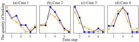
To verify that the model is effective in capturing future trends, we selected samples from the dataset with different trends for validation. As shown in Figure 4, the trend varies from sample to sample event for the same event impact: some hotels reached their peak in the early stages of the holiday and showed an overall downward trend (Figure 4 (a), (c)); some hotels had high traffic in the middle holiday period and showed an overall mountain shape (Figure 4 (b), (d)). The predicted trend of CRAFT is also not constant but changes with the actual trend of the sample, which indicates the reliability of CRAFT.
In addition, we present the hyperparameter analysis and complexity analysis in Appendix E in our full paper [Zhang et al., 2025].
5.3 Online A/B Test
To further verify the performance of CRAFT in the real online environment, we apply CRAFT to holiday inventory negotiations. In the real application, we need to predict the hotel sales before holidays, and business developers (BD) will check whether the inventory is sufficient based on the prediction results of our model. If not, they will negotiate with the hotel in advance based on the prediction results to give more inventory. We select the MQ-RNN as the baseline and utilize IWR and PHDI metrics to measure the overall impact of different models. The definition of IWR and PHDI refers to Appendix B.4 in our full paper [Zhang et al., 2025]. IWR and PHDI are defined according to specific scenarios and are the most concerned metrics in BD negotiations. Moreover, as we cannot equally assign daily traffic to each model, such as testing personalized recommendation systems, we randomly divided the hotels into two groups for the MQ-RNN and CRAFT models.
| Holiday | IWR * | PHDI† | ||
|---|---|---|---|---|
| MQ-RNN | CRAFT | MQ-RNN | CRAFT | |
| 2023 Mid-autumn | 0.0513 | 0.0306 | 0.3659 | 0.2983 |
| 2023 National Day | 0.0534 | 0.0311 | 0.3694 | 0.2990 |
| 2024 New Year's Day | 0.0601 | 0.0354 | 0.3661 | 0.3093 |
| 2024 Spring Festival | 0.0583 | 0.0337 | 0.3655 | 0.3047 |
Table 4: Online A/B test result during holiday.
For both the IWR and PHDI metrics, the smaller the value, the better the model performance. The online A/B test results are shown in Table 4. Compared with MQ-RNN, CRFAT achieves significant improvement on these two metrics. Indeed, based on the data from four holidays, CRAFT method has an average improvement of 0.0231 and an improvement rate of 41.35% on the IWR metric. On the PHDI metric, the improvement value and improvement rate are 0.0639 and 17.42%, respectively. The results above illustrate the effectiveness of CRAFT in the real application.
6 Conclusion
In this paper, inspired by real-world application, we define Cross-Future Behavior (CFB). CFB is a kind of features that occur before the current time but take effect in the future, containing true information related to future events. For the application of CFB in the TSF, we propose an improved method, named Cross-Future Behavior Awareness based Time Series Forecasting method (CRAFT). CRAFT regards the trend of CFB as prior information to predict the trend of target time series data. We conduct experiments on real-world dataset. Experiments on both offline and online tests demonstrate the effectiveness of CRAFT. However, this paper only conduct experiments on our dataset as the current public available dataset (e.g., ETT [Zhou et al., 2021], ECL 1 , Weather 2 ) does not contain the CFB feature or similar feature. In the future, we will further collect related data to form a series benchmark dataset. Moreover, we will continue to generalize the definition of CFB to enable CRAFT method to be applied more broadly.
1 ECL dataset was acquired at https://archive.ics.uci.edu/ml/ datasets/ElectricityLoadDiagrams20112014.
2 Weather dataset was acquired at https://www.ncei.noaa.gov/ data/local-climatological-data/.
Acknowledgments
This work is supported by Natural Science Foundation of China (No.62302487), AI Dream Project (No.SZSM202402), and Jinan Social and People's Livelihood Major Project (No.202317014).
Contribution Statement
- *: Yingwei Zhang and Ke Bu contributed equally to this work and share first authorship. †: Detao Lv is the corresponding author responsible for correspondence.
@inproceedings{ijcai2025p785,
  title     = {CRAFT: Time Series Forecasting with Cross-Future Behavior Awareness},
  author    = {Zhang, Yingwei and Bu, Ke and Zhuang, Zhuoran and Xie, Tao and Yu, Yao and Li, Dong and Guo, Yang and Lv, Detao},
  booktitle = {Proceedings of the Thirty-Fourth International Joint Conference on
               Artificial Intelligence, {IJCAI-25}},
  publisher = {International Joint Conferences on Artificial Intelligence Organization},
  editor    = {James Kwok},
  pages     = {7056--7064},
  year      = {2025},
  month     = {8},
  note      = {Main Track},
  doi       = {10.24963/ijcai.2025/785},
  url       = {https://doi.org/10.24963/ijcai.2025/785},
}
TY - CPAPER TI - CRAFT: Time Series Forecasting with Cross-Future Behavior Awareness AU - Zhang, Yingwei AU - Bu, Ke AU - Zhuang, Zhuoran AU - Xie, Tao AU - Yu, Yao AU - Li, Dong AU - Guo, Yang AU - Lv, Detao T2 - Proceedings of the Thirty-Fourth International Joint Conference on Artificial Intelligence, IJCAI-25 PB - International Joint Conferences on Artificial Intelligence Organization PY - 2025 SP - 7056 EP - 7064 DO - 10.24963/ijcai.2025/785 UR - https://doi.org/10.24963/ijcai.2025/785 ER -Copied
Machine-readable versions of this paper, for tools and AI agents:





