Federated Stochastic Bilevel Optimization with Fully First-Order Gradients

1 Introduction

In this paper, we focus on the following federated stochastic bilevel optimization (FedSBO) problem:

Here, g(x, y) ≜ 1N ∑Nn=1 g(n) (x, y) denotes the lowerlevel loss function, where g(n) (x, y) = E[g(n) (x, y; ξ (n) )] denotes the lower-level loss function on the n-th device, and f(x, y∗ (x)) ≜ 1N ∑Nn=1 f (n) (x, y∗ (x)) represents the upper-level loss function, where f (n) (x, y∗ (x)) = E[f (n) (x, y∗ (x); ξ (n) )] represents the upper-level loss function on the n-th device. Throughout this paper, we assume that the upper-level loss function is nonconvex with respect to both variables and the lower-level loss function is strongly convex with respect to y, which is a commonly used assumption in the existing literature [Ghadimi and Wang, 2018; Ji et al., 2021; Chen et al., 2021; Tarzanagh et al., 2022].

∗Corresponding author

The stochastic bilevel optimization problem has attracted increasing attention recently because many machine learning models belong to this class of optimization problem, such as model-agnostic meta-learning [Finn et al., 2017], hyperparameter optimization [Ji et al., 2021], neural architecture search [Liu et al., 2018], etc. To solve the stochastic bilevel optimization problem, numerous optimization algorithms [Ghadimi and Wang, 2018; Ji et al., 2021; Chen et al., 2021; Hong et al., 2020; Khanduri et al., 2021; Yang et al., 2021; Guo and Yang, 2021; Dagr´eou et al., 2022; Dagr´eou et al., 2024] have been developed in the single machine setting in the past few years. However, enabling federated learning for the stochastic bilevel optimization problem is much more challenging than the standard single-level optimization problem. Specifically, as shown in Eq. (1), the upper-level problem on each device depends on the optimal solution y∗ (x) of the global lower-level problem. As a result, computing the stochastic hypergradient for the upperlevel loss function on each device requires the global Jacobian and Hessian matrices, introducing significant challenges for local computation and global communication.

In recent years, numerous efforts [Gao, 2022; Tarzanagh et al., 2022; Li et al., 2024; Yang et al., 2024; Huang et al., 2023] have been made to address the unique challenges in FedSBO problems. For example, [Gao, 2022] developed a local stochastic bilevel gradient descent with momentum algorithms under the homogeneous setting, which can remove the dependence on global Jacobian and Hessian matrices due to the homogeneous data distribution. [Tarzanagh et al., 2022] proposed FedNEST in the heterogeneous setting. It employs the Neumann series expansion approach in an inner loop to estimate Hessian-inverse-vector product. However, this method suffers from a large communication complexity because it requires to communicate every intermediate Hessian-inverse-vector product in that inner loop. [Li et al., 2024] proposed a single-loop algorithm to address the issue of large communication complexity. In particular, it introduces an additional gradient descent procedure to replace the Neumann series expansion approach to estimate the Hessian inverse vector product.

Nevertheless, the aforementioned federated stochastic bilevel optimization algorithms still suffer from high computation costs. Specifically, those algorithms need to compute the second-order Jacobian and Hessian matrices. It is computationally expensive, especially when the problem is high-dimensional. In fact, to avoid computing the secondorder Jacobian and Hessian matrices, [Kwon et al., 2023; Shen and Chen, 2023; Kwon et al., 2024; Chen et al., 2023] developed a fully first-order method in the single-machine setting. Specifically, [Kwon et al., 2023] converts the bilevel optimization problem into a single-level one, and then only the first-order gradient is required to solve it, significantly reducing computational costs. More specifically, [Kwon et al., 2023] converts the lower-level optimization problem as a constraint and then leverages the penalty approach to further convert it to an unconstrained minimax optimization problem, which can be solved by the first-order stochastic gradient descent ascent algorithm. Inspired by this, we aim to develop an efficient federated stochastic bilevel optimization algorithm that uses only first-order gradients to address the aforementioned challenges. However, developing first-order methods for the FedSBO problem in Eq. (1) presents unique challenges, which are outlined below.

• First, existing first-order methods [Kwon et al., 2023] for the single-machine setting employ the iterationdependent learning rate to guarantee convergence. However, this strategy is not practical in federated learning. Specifically, from the iteration-dependent learning rate, the participating device is able to infer the current training stage, which could be used to attack the training procedure by attackers. Therefore, it is necessary to develop a constant learning rate to avoid this problem while guaranteeing convergence.
• Second, existing first-order methods [Kwon et al., 2023] under the single-machine setting employ a two-timescale learning rate to guarantee convergence. Specifically, some variables have an order-wise larger learning rate than the others. This kind of learning rate is difficult to tune for practical federated learning practitioners. Thus, it is necessary to propose a singletimescale learning rate to make it easy to tune while ensuring convergence.
• Third, the first-order method under the single-machine setting requires a penalty hyperparameter to guarantee convergence. However, it is unclear how this penalty hyperparameter affects the consensus error in federated learning. Specifically, it is unclear whether the impact of the penalty hyperparameter on the consensus error will lead to a slower convergence rate. Therefore, it is necessary to establish the theoretical convergence rate, revealing how the penalty hyperparameter affects the consensus error and the convergence rate in federated learning.

To address the aforementioned unique challenges, we develop a novel federated stochastic variance-reduced bilevel gradient descent algorithm with fully first-order oracles. Specifically, on the algorithm design side, we develop a novel single-timescale constant learning rate, where we demonstrate how this new learning rate depends on the penalty hyperparameter. On the theoretical analysis side, we propose a novel strategy to establish the convergence rate of our algorithm. In particular, we develop a novel potential function for convergence analysis, where we demonstrate how to combine different components together with carefully designed coefficients. With these novel algorithmic and theoretical designs, our algorithm can achieve the O( 1 Nϵ5 ) convergence rate to obtain the ϵ-accuracy solution, which indicates the linear speedup with respect to the number of devices N. Finally, extensive experimental results confirm the efficacy of our new algorithm. In summary, our paper has made the following contributions.

• We develop a novel federated stochastic variancereduced bilevel gradient descent algorithm, which uses the fully first-order gradient and the single-timescale constant learning rate. To the best of our knowledge, this is the first time a single-timescale constant learning rate has been shown to be applied to the first-order bilevel optimization algorithms.
• We establish the convergence rate of our algorithm, where we demonstrate how to use a potential function to combine different estimation errors together with carefully designed coefficients. As far as we know, this is the first work to provide convergence guarantees for firstorder federated bilevel optimization algorithms with the single-timescale constant learning rate .
• Our extensive experimental results on various tasks confirm the efficacy of our algorithm, i.e., our new algorithm is more computationally efficient than existing secondorder methods.

2 RelatedWorks

2.1 Stochastic Bilevel Optimization

Since the upper-level loss function depends on the optimal solution of the lower-level optimization problem, the hypergradient of the upper-level loss function needs to compute ∂y∗ (x)/∂x, which brings unique challenges for optimizing this class of optimization problems. Specifically, computing ∂y∗ (x)/∂x depends on Jacobian and Hessian inverse matrices. To compute them, many efforts [Ghadimi and Wang, 2018; Ji et al., 2021; Chen et al., 2021; Hong et al., 2020; Khanduri et al., 2021; Yang et al., 2021; Guo and Yang, 2021; Dagr´eou et al., 2022; Chu et al., 2024; Dagr´eou et al., 2024] have been made in the single machine setting recently. For example, [Ghadimi and Wang, 2018] proposed using the Neumann series expansion approach to approximate the Hessianinverse-vector product, based on which the convergence rate of the stochastic gradient descent is established. In this direction, several improved algorithms have been developed. For example, [Ji et al., 2021] developed a mini-batch stochastic gradient descent method to improve the convergence rate with a large batch size. [Hong et al., 2020] studied the convergence rate of the stochastic gradient descent with a two-timescale learning rate. [Chen et al., 2021] established the convergence rate of the stochastic gradient descent with an alternating update strategy. To further improve the convergence rate, [Khanduri et al., 2021; Yang et al., 2021;

Guo and Yang, 2021] introduces the variance reduction techniques [Cutkosky and Orabona, 2019; Fang et al., 2018; Nguyen et al., 2017] into stochastic bilevel optimization, whose convergence rate O(ϵ-3 ) can match their counterparts for the single-level optimization problem. In addition to the Neumann series expansion approach, there exists another approach for estimating the hypergradient. Specifically, the Hessian-inverse-vector product is viewed as the optimal solution of a quadratic optimization problem, and then an additional gradient descent procedure is introduced to estimate the Hessian-inverse-vector product. Based on this approach, a couple of algorithms have been developed. For example, [Dagr´eou et al., 2022; Chu et al., 2024; Dagr´eou et al., 2024] combined it with variance reduction techniques, whose convergence rates O(ϵ-3 ) can also match their counterparts for the single-level optimization problem.

Since the aforementioned approaches need to compute the second-order Jacobian and Hessian inverse matrices, [Kwon et al., 2023; Shen and Chen, 2023] developed the fully firstorder method to address this issue. In particular, they transformed the lower-level optimization problem as a constraint and then used the penalty approach to further convert it as an unconstrained minimax optimization problem. However, the penalty hyperparameter significantly affects the convergence rate. For example, [Kwon et al., 2023] shows that the standard stochastic gradient descent ascent algorithm can only achieve the convergence rate of O(ϵ-7 ) and can be improved to O(ϵ-5 ) with the variance reduction technique. However, these methods do not require computation of the second-order Jacobian and Hessian inverse matrices. As a result, their practical performance is more efficient in terms of running time, especially when the problem is high-dimensional.

2.2 Federated Stochastic Bilevel Optimization

To enable distributed optimization for stochastic bilevel optimization problems, numerous algorithms [Gao, 2022; Tarzanagh et al., 2022; Li et al., 2024; Yang et al., 2024; Huang et al., 2023; Gao et al., 2023; Zhang et al., 2023] have recently been developed. For example, based on the Neumann series expansion approach, [Gao, 2022] developed local stochastic bilevel gradient descent with momentum algorithms under the homogeneous setting, which only need to communicate two variables and their gradient estimators. Its communication complexity O(ϵ-1 ) can match its counterpart for the single machine setting. [Tarzanagh et al., 2022] proposed FedNEST for the heterogeneous setting, where every intermediate Hessian-inverse-vector product in the the Neumann series expansion approach should be communicated, leading to a large communication complexity. Later, [Huang et al., 2023] developed the FedMBO algorithm, which does not need to communicate the intermediate Hessian-inverse-vector product. However, the upperlevel variable in FedMBO needs to be communicated in every iteration, which also leads to a large communication complexity. Based on the other approach for estimating Hessianinverse-vector product, [Li et al., 2024] developed a federated stochastic bilevel optimization algorithm with the variance reduction technique, whose communication complexity can match that of its counterpart for the single-level problem.

However, all these existing algorithms need to compute the second-order Jacobian and Hessian matrices, which is computationally expensive for high-dimensional problems. As far as we know, there do not exist first-order federated bilevel optimization algorithms. Note that a concurrent work [Yang et al., 2025] appeared online after we submitted our paper to IJCAI, and it has a worse convergence rate O(ϵ-7 ).

3 AlgorithmDesign

3.1 ProblemDefinition

According to [Kwon et al., 2023], Eq. (1) can be converted to a constrained optimization problem as follows:

Then, by leveraging the penalty approach, this constrained optimization problem can be converted to an unconstrained minimax optimization problem as follows:

where λ > 0 is the penalty hyperparameter. Denoting

where y∗λ (x) = argminy∈Rdy f(x, y) + λ(g(x, y) - g(x, y∗ (x))), existing works [Kwon et al., 2023] have shown that L∗λ (x) is a good approximation to L(x) when given an appropriate penalty hyperparameter λ.

Based on this reformulation, we can solve Eq. (1) by optimizing the following minimax problem:

Obviously, the gradients ∇xL(n) λ (x, y, z), ∇yL(n) λ (x, y, z), and ∇zL(n) λ (x, y, z) on the n-th device do not depend on the second-order Jacobian and Hessian matrices. Thus, Eq. (4) can be solved efficiently.

3.2 Our Algorithm

To solve Eq. (4), we develop a novel federated stochastic variance-reduced bilevel gradient descent algorithm with fully first-order oracles (FedSVRBGD-FO) in Algorithm 1. Specifically, in the t-th iteration, device n computes the stochastic variance-reduced gradient for each component of ∇xL(n) λ (x, y, z) as follows:

.

Algorithm 1 FedSVRBGD-FO

Input: x0, y0, z0, η > 0, αx > 0, αy > 0, αz > 0, βx > 0, βy > 0, βz > 0.

• 1: Initialization when t = 0: compute the stochastic gradient with a mini-batch of samples where the batch size is B:

• 2: for t = 0, · · · , T -1, each device n do
• 3: Update x: x(n) t+1 = x(n) t -αxηm(n) x,t ,
• 4: Update y : y(n) t+1 = y(n) t -αyηm(n) y,t ,
• 5: Update z: z(n) t+1 = z(n) t -αzηm(n) z,t ,
• 6: Update the variance-reduced gradient m(n)
• x,t+1 :

• 7: Update the variance-reduced gradient m(n)

• y,t+1 : t+1 ) ,
• 8: Update the variance-reduced gradient m(n) z,t+1 : w(n) 1,t+1 = (1 - βzη2 )(w(n) 1,t -∇2g(n) (x(n) t , z(n) t ; ξ (n) t+1 )) + ∇2g(n) (x(n) t+1 , z(n) t+1 ; ξ (n) t+1 ) , m(n) z,t+1 = λw(n) 1,t+1 ,
• 9: if mod(t + 1, p) == 0 then

• 11: end if

12: end for

where η > 0 is the learning rate and βx > 0 is a constant hyperparameter, which satisfies βxη2 < 1. Then, our algorithm composes the variance-reduced gradient estimator for ∇xL(n) λ (x, y, z) as follows:

This gradient estimator is then used to update the local variable as follows:

where αx > 0 is a constant hyperparameter. Then, at every p iterations, where p > 1, the local variable x(n) t+1 and gradient estimators u(n) 1,t+1 , u(n) 2,t+1 , u(n) 3,t+1 are uploaded to the central server and then reset to the global ones, which is shown in Step 9 in Algorithm 1. The other two variables are updated in the same way.

It is worth noting that the learning rate η and the associated hyperparameters αx, αy, αz in our Algorithm 1 are constant, rather than iteration-dependent as existing methods in the single-machine setting.

4 Convergence Analysis

4.1 Assumption

To establish the convergence rate of our Algorithm 1, we introduce the following assumptions that are commonly used in existing work [Kwon et al., 2023; Chen et al., 2023].

Assumption 4.1. For n ∈ {1, · · · ,N}, the upper-level function f (n) (·, ·) is Lf -smooth in expectation where Lf > 0 is a constant, and it is Cf -Lipschitz with respect to the second variable in expectation.

Assumption 4.2. For n ∈ {1, · · · ,N}, the lower-level function g(n) (·, ·) is Lg,1-smooth in expectation where Lg,1 > 0 is a constant and ∇2 g(·, ·) is Lg,2-Lipschitz in expectation where Lg,2 > 0 is a constant.

Assumption 4.3. For n ∈ {1, · · · ,N}, the lower-level function g(n) (·, ·) is µ-strongly-convex with respect to the second variable.

• 0 ) ,

Based on Assumptions 4.1-4.3, [Kwon et al., 2023] shows that Lλ(x, y, z) is λµ 2 -strongly-convex in y when λ > 2Lf µ .

Assumption 4.4. The stochastic gradients of the loss functions at the upper and lower levels have an upper bounded variance σ2 where σ > 0 is a constant.

Assumption 4.5. The data distribution between workers is heterogeneous and the upper-level and lower-level gradients satisfy the following conditions:

where δ > 0 is a constant, x ∈ Rdx , and y ∈ Rdy .

Following [Chen et al., 2023], we introduce the following definition.

Definition 4.6. Given Assumptions 4.1-4.3, we denote ℓ = max{Cf , Lf , Lg,1, Lg,2} and κ = ℓ/µ.

With the aforementioned assumptions and definitions, the following lemma shows how well L∗λ (x) approximates L(x).

Lemma 4.7. [Chen et al., 2023; Kwon et al., 2023] Given Assumptions 4.1-4.3, by setting λ > 2Lf µ , thenL∗λ (x) satisfies the following conditions:

• ∇L∗λ (x) is L-Lipschitz, where L = O(ℓκ3 );
• ∥∇L∗λ (x) -∇L(x)∥ = O(ℓκ3 /λ) for any x ∈ Rdx ;
• |L∗λ (x) -L(x)| = O(ℓκ2 /λ) for any x ∈ Rdx .

4.2 Convergence Rate

Based on Assumptions 4.1-4.5, we established the convergence rate of our algorithm below, whose proof can be found in Appendix.

O ( κ Nϵ ), B = O ( κ6 Nϵ3 ), and T = O ( κ10 Nϵ5 can achieve the ϵ-accuracy solution as follows:

Remark 4.9. The complexity of the iteration T = O ( κ10 Nϵ5 ) indicates that our algorithm can achieve a linear speedup with respect to the number of devices N. To the best of our knowledge, this is the first time that the first-order algorithm can achieve the linear speedup for federated bilevel optimization problems. Moreover, when N = 1, i.e., the single-machine setting, our convergence rate can match that of the singlemachine counterpart in [Kwon et al., 2023]. Furthermore, the communication complexity of Algorithm 1 is Tp = O ( κ9 ϵ4 ).

Remark 4.10. The existing method [Kwon et al., 2023] under the single-machine setting employs a time-dependent learning rate. For example, the learning rate in the t-th iteration for x is of the order of O(t-3/5 ). On the contrary, our Algorithm 1 employs a constant learning rate η that is independent of the current iteration. Moreover, [Kwon et al., 2023] employs a two-timescale learning rate. Specifically, the learning rate for x is O(t-3/5 ), while that for z is O(t-2/5 ). Then, limt→∞ t-3/5 /t-2/5 = 0. In contrast, the learning rate for three variables in Algorithm 1, i.e., αxη, αyη, and αzη, are in the same timescale 1 . Therefore, our learning rate setting is easier to tune in practice.

4.3 Proof Sketch

To establish the convergence of Algorithm 1, we develop a novel potential function as follows:

where {ci}8i=1 are positive coefficients.

A key design in our potential function is that c1 and c2 are associated with λ while c4, c5, c7, and c8 are associated with λ2 . As such, all coefficients {ci}8i=1 are independent of the penalty parameter λ. Otherwise, {ci}8i=1 will depend on λ, which will further affect the variance term and then result in a worse convergence rate. For example, as shown in Eq. (68), the coefficient {ci}8i=3 affects the terms regarding the variance in the last line. If they depended on the penalty parameter, the learning rate η has to be much smaller to control the variance term. For example, when c4 = O(λ2 ), η should be as small as O(ϵ6 ) because of λ = O( 1ϵ ), leading to a much slower convergence rate.

Based on this potential function, we first establish the upper bound for each term of this potential function in the Appendix A.1 and then identify the coefficient {ci}8i=1 in Appendix A.2 to eliminate all their associated terms in the upper bound of Pt+1 - Pt, resulting in Eq. (131). Then, we can establish the convergence rate of our Algorithm 1.

1 In this paper, the same timescale refers to having the same order with respect to ϵ or the number of iterations.

Moreover, a key step for establishing the final convergence rate is to bound the consensus error in the following lemma, whose proof can be found in Appendix A.1.

In this lemma, we reveal how the penalty hyperparameter λ and the communication period p affect the consensus error. With such a lemma, we can then establish the convergence rate of our Algorithm 1.

5 Experiments

In this section, we evaluate the performance of our Algorithm 1 on the commonly used benchmark task: hyperparameter optimization and hyper-representation learning.

5.1 Hyperparameter Optimization

In the experiment, we apply Algorithm 1 to the following hyperparameter optimization problem:

where the lower-level problem is to learn the parameter y ∈ Rd×c of the logistic regression model with the training set {(a(n) t,i , b(n) t,i )}m(n) i=1 , the upper-level problem learns the the regularization coefficient x ∈ Rd with the validation set {(a(n) v,i , b(n) v,i )}m(n) i=1 .

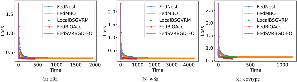
In this experiment, we used three benchmark datasets: a9a, w8a, covtype, which are obtained from LIBSVM datasets 2 . Here, 10% of the samples are randomly selected as the test set. For the remaining samples, 70% of them are randomly selected as the training set and the others are used as the validation set. The training and validation sets are then randomly distributed to eight workers. The batch size for each worker is set to 10 in this experiment. To verify the performance of our Algorithm 1, we compare it with four state-of-the-art second-order methods: FedNEST [Tarzanagh et al., 2022], FedMBO [Huang et al., 2023], LocalBSGVRM [Gao, 2022], and FedBiOAcc [Li et al., 2024]. In our experiment, we set the solution accuracy ϵ to 0.1. Then, according to the theoretical results in [Tarzanagh et al., 2022; Huang et al., 2023; Gao, 2022; Li et al., 2024], the learning rate of FedNEST and FedMBO is set to ϵ2 , while that of LocalBSGVRM and FedBiOAcc is set to ϵ. Regarding our method, according to Theorem 4.8, we set the learning rate η to ϵ2 , the coefficient αx = αy = αz = ϵ, and the penalty λ = 5/ϵ. Moreover, for all methods using the momentum-based variance reduction technique, we set the the coefficient of the momentum to 0.1. Then, we run all experiments on a workstation with 4 NVIDIA A5000 GPU cards, each of which accommodates two threads to simulate eight workers.

2 https://www.csie.ntu.edu.tw/∼cjlin/libsvmtools/datasets/

In Figure 1, we plot the upper-level loss function value versus the running time (seconds). Specifically, to make a fair comparison, we ran all methods to update x for 16,000 iterations on all datasets. The communication period is set to 4 in this experiment. From Figure 1, we can find that our algorithm requires much less time to converge than all baseline methods. This confirms the advantage of using the fully firstorder gradient in practical applications.

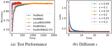
In addition, in Figure 2(a), we plot the accuracy in the test set versus the running time for the a9a dataset. In Figure 2(a), we can still find that our algorithm uses much less time to achieve almost the same accuracy as the baseline methods, further confirming the efficacy of using fully first-order gradients for federated bilevel optimization.

Because the learning rate and penalty parameter are set according to the accuracy of the solution ϵ as suggested by Theorem 4.8, we added an additional experiment to show the influence of ϵ on the convergence rate, which is shown in Figure 2(b). It can be observed that a smaller ϵ leads to a slower convergence rate. The reason is that a smaller ϵ results in a smaller learning rate as shown in Theorem 4.8, slowing the convergence.

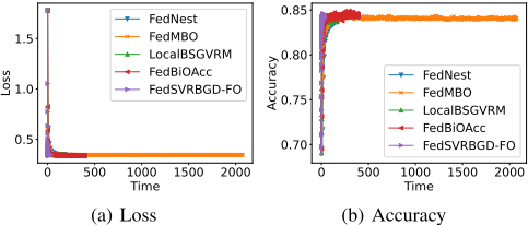
Furthermore, to verify the impact of the communication period on convergence performance, we performed an additional experiment with p = 16. In Figure 3, we plot the upper-level loss function value versus the running time in Figure 3(a) and plot the test accuracy in Figure 3(b). Note that FedNest becomes more efficient than FedBiOAcc because it computes the second-order Hessian and Jacobian matrices in each communication round, rather than each iteration. Thus, it computes second-order information less frequently when the communication period becomes large. However, we can still find that our algorithm needs less time to converge than all baseline methods when the communication period is 16.

5.2 Hyper-representation Learning

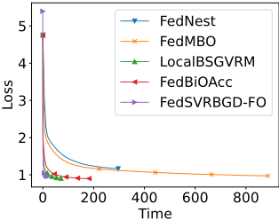
To further verify the performance of our algorithm, we apply our algorithm to the hyper-representation learning task as [Tarzanagh et al., 2022]. Specifically, given a deep neural network, the upper-level problem learns the weight of hidden layers, while the lower-level problem learns the weight of the classifier. As such, the upper-level problem is nonconvex and the lower-level one is strongly convex when using the cross-entropy loss function with ℓ2-norm regularization for the classifier's weight. In our experiment, we used a fully connected two-layer neural network. Its dimensionality of the input, hidden, and output layer is 54, 30, and 7, respectively. The dataset is covtype, which has seven classes. The batch size is 100. The communication period p = 4. All the other settings are the same as the first experiment.

In Figure 4, we plot the loss function value versus the running time (seconds) for the hyper-representation task. It can be seen that our algorithm converges much faster than all baseline methods in terms of running time, which further confirms the advantages of using the first-order gradient over the second-order ones.

6 Conclusions

In this paper, we develop a novel federated stochastic bilevel optimization algorithm based on the fully first-order gradient. In particular, each work only needs to compute the first-order stochastic variance-reduced gradient to update the upper- and lower-level variables. This can significantly save running time because our algorithm does not need to compute the second-order Hessian and Jacobian matrices. Moreover, we developed a novel single-timescale constant learning rate to coordinate the update of different variables and presented a novel strategy to establish the convergence rate of our algorithm. The extensive experimental results confirm the efficacy of our algorithm.

Acknowledgments

1. Zhang and H. Gao were partially supported by U.S. NSF CAREER 2339545, NSF IIS 2416607, NSF CNS 2107014.