
Asset Pricing with Contrastive Adversarial Variational Bayes
Proceedings of the Thirty-Fourth International Joint Conference on Artificial Intelligence. Main Track. Pages 7572-7579.
https://doi.org/10.24963/ijcai.2025/842
Keywords
- Uncertainty in AI: UAI: Applications
- Multidisciplinary Topics and Applications: MTA: Finance
- Data Mining: DM: Applications
Abstract
Machine learning techniques have gained considerable attention in the field of empirical asset pricing. Conditioning on a broad set of firm characteristics, one of the most popular no-arbitrage workhorses is a nonlinear conditional asset pricing model that consists of two modules within a neural network structure, i.e., factor and beta estimates, for which we propose a novel contrastive adversarial variational Bayes (CAVB) framework. To exploit the factor structure, we employ adversarial variational Bayes that transforms the maximum-likelihood problem into a zero-sum game between a variational autoencoder (VAE) and a generative adversarial network (GAN), where an auxiliary discriminative network brings in arbitrary expressiveness to the inference model. To tackle the problem of learning indistinguishable feature representations in the beta network, we introduce a contrastive loss to learn distinctive hidden features of the factor loadings in correspondence to conditional quantiles of return distributions. CAVB establishes a robust relation between the cross-section of asset returns and the common latent factors with nonlinear factor loadings. Extensive experiments show that CAVB not only significantly outperforms prominent models in the existing literature in terms of total and predictive R-squares, but also delivers superior Sharpe ratios after transaction costs for both long-only and long-short portfolios.
- [Bryzgalova et al., 2023a] Svetlana Bryzgalova, Jiantao Huang, and Christian Julliard. Bayesian solutions for the factor zoo: We just ran two quadrillion models. The Journal of Finance, 78(1):487-557, 2023.
- [Bryzgalova et al., 2023b] Svetlana Bryzgalova, Markus Pelger, and Jason Zhu. Forest through the trees: Building cross-sections of stock returns. The Journal of Finance, Forthcoming, 2023.
- [Chatigny et al., 2021] Philippe Chatigny, Ruslan Goyenko, and Chengyu Zhang. Asset pricing with attention guided deep learning. Available at SSRN 3971876, 2021.
- [Chen et al., 2024] Luyang Chen, Markus Pelger, and Jason Zhu. Deep learning in asset pricing. Management Science, 70(2):714-750, 2024.
- [Cochrane, 2011] John H Cochrane. Presidential address: Discount rates. The Journal of Finance, 66(4):1047-1108, 2011.
- [Duan et al., 2022] Yitong Duan, Lei Wang, Qizhong Zhang, and Jian Li. FactorVAE: A probabilistic dynamic fac- tor model based on variational autoencoder for predicting cross-sectional stock returns. In Proceedings of the AAAI Conference on Artificial Intelligence, volume 36, pages 4468-4476, 2022.
- [Duan et al., 2025] Yitong Duan, Weiran Wang, and Jian Li. Factorgcl: A hypergraph-based factor model with tempo- ral residual contrastive learning for stock returns predic- tion. In Proceedings of the AAAI Conference on Artificial Intelligence, volume 39, pages 173-181, 2025.
- [Freyberger et al., 2020] Joachim Freyberger, Andreas Neuhierl, and Michael Weber. Dissecting characteristics nonparametrically. The Review of Financial Studies, 33(5):2326-2377, 2020.
- [Gu et al., 2021] Shihao Gu, Bryan Kelly, and Dacheng Xiu. Autoencoder asset pricing models. Journal of Economet- rics, 222(1):429-450, 2021.
- [He et al., 2020] Kaiming He, Haoqi Fan, Yuxin Wu, Sain- ing Xie, and Ross Girshick. Momentum contrast for un- supervised visual representation learning. In Proceedings of the IEEE/CVF Conference on Computer Vision and Pat- tern Recognition, pages 9729-9738, 2020.
- [Jia et al., 2024] Yulong Jia, Guanxing Li, Ganlong Zhao, Xiangru Lin, and Guanbin Li. GraphVAE: Unveiling dy- namic stock relationships with variational autoencoder- based factor modeling. In Proceedings of the 33rd ACM International Conference on Information and Knowledge Management, pages 3807-3811, 2024.
- [Kelly et al., 2019] Bryan T Kelly, Seth Pruitt, and Yinan Su. Characteristics are covariances: A unified model of risk and return. Journal of Financial Economics, 134(3):501- 524, 2019.
- [Koenker and Bassett Jr, 1978] Roger Koenker and Gilbert Bassett Jr. Regression quantiles. Econometrica: Journal of the Econometric Society, pages 33-50, 1978.
- [Kozak et al., 2018] Serhiy Kozak, Stefan Nagel, and Shri- hari Santosh. Interpreting factor models. The Journal of Finance, 73(3):1183-1223, 2018.
- [Kozak et al., 2020] Serhiy Kozak, Stefan Nagel, and Shri- hari Santosh. Shrinking the cross-section. Journal of Fi- nancial Economics, 135(2):271-292, 2020.
- [Mescheder et al., 2017] Lars Mescheder, Sebastian Nowozin, and Andreas Geiger. Adversarial varia- tional Bayes: Unifying variational autoencoders and generative adversarial networks. In International Con- ference on Machine Learning, pages 2391-2400.
- PMLR, 2017.
- [Shi et al., 2025] Hao Shi, Weili Song, Xinting Zhang, Jiahe Shi, Cuicui Luo, Xiang Ao, Hamid Arian, and Luis Angel Seco. AlphaForge: A framework to mine and dynami- cally combine formulaic alpha factors. In Proceedings of the AAAI Conference on Artificial Intelligence, volume 39, pages 12524-12532, 2025.
- [Vaswani et al., 2017] Ashish Vaswani, Noam Shazeer, Niki Parmar, Jakob Uszkoreit, Llion Jones, Aidan N Gomez, Łukasz Kaiser, and Illia Polosukhin. Attention is all you need. Advances in Neural Information Processing Sys- tems, 30, 2017.
- [Wei et al., 2023] Zikai Wei, Anyi Rao, Bo Dai, and Dahua Lin. HireVAE: an online and adaptive factor model based on hierarchical and regime-switch VAE. In Proceedings of the Thirty-Second International Joint Conference on Arti- ficial Intelligence, pages 4903-4911, 2023. IJCAI
- [Xiang et al., 2024] Quanzhou
- Xiang, Zhan Chen, Qi Sun, and Rujun Jiang. RSAP-DFM: regime-shifting adaptive posterior dynamic factor model for stock returns predic- tion. In Proceedings of the Thirty-Third International Joint Conference on Artificial Intelligence, pages 6116-6124, 2024. IJCAI
- [Yang et al., 2024] Xuanling Yang, Zhoufan Zhu, Dong Li, and Ke Zhu. Asset pricing via the conditional quantile variational autoencoder. Journal of Business & Economic Statistics, 42(2):681-694, 2024.
References were extracted automatically from the PDF and may contain errors.
Full text extracted automatically from the PDF; figures, tables and equations may differ. The PDF is the version of record.
1 Introduction
Factor models have become the workhorse for predicting asset returns using conditional information such as asset characteristics. In particular, dynamic factor models (DFM) are broadly employed. [Duan et al., 2022] incorporate a variational autoencoder (VAE) into a DFM and propose a priorposterior learning scheme for return prediction. [Wei et al., 2023] design a hierarchical VAE-based DFM, which adaptively captures the regime-switching spatio-temporal relations in return prediction. [Xiang et al., 2024] also emphasize the importance of regime switches in the DFM and rely on adversarial posterior factors to correct mapping deviations from prior factors. [Jia et al., 2024] introduce adaptive graphs into a VAE-based factor model to capture dynamic asset relations. [Duan et al., 2025] propose a hypergraph-based DFM with temporal contrastive learning that extracts additional hidden factors from residual information beyond the prior factors. [Shi et al., 2025] design a surrogate model to predict fitness scores for factor mining and dynamically adjust factor weights in factor combinations. However, these papers ignore the well-known factor structure embedded in asset returns, which is the focus of this study.
A general factor model for empirical asset pricing assumes that the excess return ri,t of asset i = 1, ...,N at time t = 1, ..., T exhibits a K-factor structure as follows:
where βi,t ∈ RK×1 is the factor loading vector that can be interpreted as the exposures to K common latent factors ft+1 ∈ RK×1 , and ϵi,t+1 is the idiosyncratic error. The empirical estimation of (1) is challenging, as the factors are unobservable or unknown.
Most existing studies prespecify factors and estimate the corresponding betas via regression. A key limitation of this approach is its reliance on prior knowledge to identify relevant factors, a challenge often addressed in the literature through portfolio sorting based on characteristics. This results in the 'factor zoo' issue in empirical asset pricing [Cochrane, 2011].
[Kozak et al., 2018] argue that given substantial commonality in the cross-section of returns, the absence of neararbitrage opportunities implies that the stochastic discount factor (SDF) for explaining the return variations can be summarized by a few dominating factors. To address the issues of conventional principal component analysis applied to asset pricing, [Kelly et al., 2019] propose the instrumented PCA (IPCA) method to estimate ft+1 as follows:
Here zi,t ∈ RP×1 is the observable characteristics of asset i with P strictly greater than K, and β(zi,t) is a linear beta function of zi,t. The dynamic factor loadings are given by β(zi,t)′ = z′i,tΓβ, where Γβ ∈ RP×K is a coefficient matrix. This setup specifies that characteristics are proxies for the sensitivities to common factors and thereby predict the average returns. Accordingly, [Kelly et al., 2019] consider characteristics as instruments in PCA and find that the IPCA model with five factors significantly outperforms competing models published previously.
Using adaptive group LASSO, [Freyberger et al., 2020] show that many of the previously identified characteristics do not offer incremental predictive information about expected returns. [Bryzgalova et al., 2023a] employ Bayesian model averaging to handle the model specification problem with weakly identified factors. These studies still fall into the category of linear models. However, [Freyberger et al., 2020] argue that the nonlinearities in characteristics are important for providing incremental information about the cross-section of expected returns. [Bryzgalova et al., 2023b] propose a splitand-select model that spans the SDF based on decision trees, and show that it outperforms random forest or conventional deep learning methods.
[Gu et al., 2021] also criticize the linearity assumption of the IPCA approach. They propose conditional autoencoder (CAE) asset pricing models that allow for a flexible nonlinear function of the covariates by applying a neural network method to learn β(zi,t). They employ the autoencoder method to compress the N-dimensional rt+1 return matrix into a K-dimensional latent factor ft+1 using a neural network g, i.e., ft+1 = g(rt+1). Then (2) is re-written in a nonlinear form as
Without an intercept, this equality respects the no-arbitrage condition. [Gu et al., 2021] apply a fully connected network to estimate the model and find that characteristics predict average returns because they help to identify the risk exposures to common latent factors rather than capture mispricings. 1 They also show that IPCA is a special case of linear CAE when the covariance matrix of the characteristics is constant. Moreover, even if the covariance matrix varies over time, the empirical results remain similar.
With the rapid development of deep learning methods, recent studies have notably improved the performance of empirical asset pricing models by enhancing the learning capability of feature representation of the latent factors and factor loadings. Similarly to [Kozak et al., 2020], who shrink redundant characteristics, [Chatigny et al., 2021] rely on the attention mechanism [Vaswani et al., 2017] to learn sparse features of a broad set of characteristics in an asset pricing model based on the high-dimensional optimization of the SDF weights. The resulting model significantly improves the performance of the baseline model without the attention mechanism.
Other research focuses on alternative training strategies. [Chen et al., 2024] suggest that, within the SDF-based asset pricing framework, the loss function of weighted moments in the sample can be interpreted as weighted mean pricing errors. With this point of view, minimizing the objective loss is equivalent to imposing the no-arbitrage restriction. They employ adversarial learning to train neural networks, i.e., generalized adversarial networks (GANs), and achieve better performance than other classical deep learning frameworks, such as feed-forward or recurrent neural networks, including long short-term memory networks.
1 Accordingly, the alpha αi = Et[ri,t+1] - Et[β′i,tft+1] can be tested against zero for mispricing.
[Yang et al., 2024] propose the conditional quantile variational autoencoder (CQVAE) network, which links the factor structure to the conditional quantiles of returns. Specifically, CQVAE learns the J quantile-dependent beta functions βj(zt) via a multi-head neural network, where j = 1, ..., J is the quantile index. Then it estimates f(rt+1) via a VAE network. Compared to the standard autoencoder network, VAE alleviates the overfitting problem of deep learning methods. As a result, the CQVAE model significantly outperforms the CAE model.
Although the CQVAE model achieves impressive results, two major challenges remain. First, while it is economically meaningful for the CQVAE to learn quantile-dependent beta functions based on conditional return distributions, there is no empirical guarantee that the factor loadings learned by the beta network differ meaningfully across quantiles. This is because the preset quantile boundaries are not conditioned on additional information, making them suboptimal from a feature clustering perspective. If certain learned beta functions are indistinguishable from each other, the model will inevitably fail to explain the cross-section of asset returns. Second, as shown in the left panel of Figure 1, it is difficult for the approximate distributions of latent factors ft+1 learned by the VAE-based inference model qϕ(ft+1|rt+1) in the CQVAE to capture the true posterior distributions, which limits the representational capability of latent factors. This is due to the limited expressiveness of the inference model, which constrains the performance of the resulting asset pricing model. Therefore, it is crucial to improve the feature extraction capacity of the factor network.
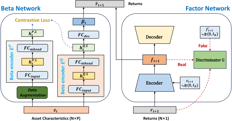
To address the above challenges, we propose a novel contrastive adversarial variational Bayes (CAVB) network to estimate (3). As shown in Figure 2, the proposed CAVB model consists of two neural network modules. The first module that improves the factor network aims to learn the common latent factors ft+1 by applying the adversarial variational Bayes (AVB) method. Especially, AVB improves the inference models qϕ(ft+1|rt+1, ϵt+1) by treating the noise ϵt as an additional input to the inference model, instead of adding it at the very end to construct the distributions in the VAE. This approach enables the inference network to learn the complex implicit probability distributions using adversarial training, which is achieved by introducing an auxiliary discriminative network as in the GAN that transforms the maximum likelihood problem into a zero-sum game where two networks contest with each other. This allows us to train the VAE with arbitrarily expressive inference models, and therefore, the representational capability of common latent factors is largely enhanced. The comparison of the conventional VAE and AVB is shown in Figure 1.
The second module of CAVB improves the beta network by introducing a contrastive learning method that focuses on extracting distinctive features for the return quantile-dependent beta functions βτ(zt). Given a set of characteristics zt as inputs, each βτ(zt) is a neural network of three fully connected layers (FCLs) with a ReLu activation function and outputs the quantile-dependent factor loadings. To enhance
(a) VAE
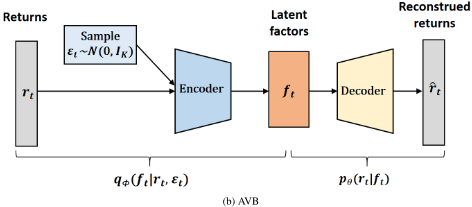
the learning capacity of distinctive features between different quantile-dependent functions, we incorporate contrastive learning into the model training process. Contrastive learning was proposed by [He et al., 2020] and aims to learn the feature representations of data by distinguishing similar data from dissimilar data through the use of appropriate positive and negative samples. To avoid learning indistinguishable feature representations for the beta functions, a contrastive loss is introduced by setting different quantile-dependent features as negative samples and those within the same conditional quantile distributions of returns as positive samples.
The remaining article is structured as follows. We present the overall architecture of the proposed CAVB model in Section 2. The architecture consists of a beta network and a factor network. In this section, we also provide details on the CAVB network training process, including contrastive and adversarial learning methods. Section 3 presents empirical studies on a comprehensive real-world dataset. Section 4 concludes.
2 Methodology
We next present the overall architecture of the proposed framework, namely, the contrastive adversarial variational Bayes (CAVB), as described in Figure 2. It consists of two modules, namely a factor network using adversarial variational Bayes (AVB) and the beta network using conditional quantile-based contrastive learning. We also provide details of their training process.
2.1 Factor Network
In the factor network, we employ AVB, as proposed by [Mescheder et al., 2017], wich unifies the VAE and GAN methods for learning the common latent factors ft. The inference model of the conventional VAE method does not produce a sufficiently rich expressiveness to capture the true posterior distributions of the latent factors. To address this issue, AVB introduces an additional auxiliary discriminative network that allows the inference model to generate arbitrarily flexible and diverse probability distributions qϕ(ft|rt). The two competing networks, GAN and VAE, rephrase the maximum-likelihood problem as a zero-sum game that allows the model to closely approximate the true posterior distribution pθ(ft|rt). In comparison with conventional VAE (see left panel of Figure 1), AVB (see right panel of Figure 1) treats noise as an additional input to the inference model, rather than adding it at the very end. This particular setup enables the inference network to learn complex implicit probability distributions via adversarial training.
The conventional VAE is trained by maximizing the evidence lower bound (ELBO) that estimates the marginal loglikelihood log pθ(rt) in
AVB shares the same objective function but is accompanied by an implicit inference model. The objective function of AVB is formally given by
where pD(rt) is the sample distribution of rt. Since VAE has an explicit Gaussian inference model of qϕ(ft|rt) parameterized by a neural network, it is easy to optimize its objective function by an appropriate re-parameterization and stochastic gradient descent (SGD). However, as shown in the right panel of Figure 1, the inference model qϕ(ft|rt) of AVB is implicit. Hence, we cannot apply the re-parameterization to calculate the termKL(qϕ(ft|rt)||pθ(ft)) in (4).
To solve this problem, we introduce a discriminative network Gψ(rt, ft) that takes the asset returns rt and common latent factors ft as inputs and gives corresponding discriminative values. The discriminative network first concatenates rt and ft, then feeds them into several linear layer blocks with residual connections, and finally outputs the discriminative values hout as follows:
where Win ∈ RD×(N+K) , W ∈ RD×D , and Wout ∈ R1×D are the matrices of weight parameters, bin ∈ RD , b ∈ RD , and bout ∈ R1 are the bias parameters, D is the hidden dimension, and ELU(·) is the exponential linear unit activation function.
The discriminative network in a standard GAN is used for judging whether the generated data are real or fake. In the proposed CAVB, we employ this type of discriminator to differentiate the pairs (rt, ft) sampled from the posterior distributions qϕ(ft|rt)pD(rt) and those sampled from the prior distributions p(ft)pD(rt). To do so, we assign the following task to the discriminator Gψ(rt, ft):
where σ is the sigmoid function. When the discriminator maximizes the objective function in (4), in the literature the optimal discriminator commonly replaces KL(qϕ(ft|rt)||pθ(ft)), and we can use
As a result, we can replace KL(qϕ(ft|rt)||pθ(ft)) by the optimal discriminator, and the objective function of AVB in (4) changes to
As shown in the right panel of Figure 1, AVB incorporates the noise ϵt ∼ N(0, I) as an additional input to the inference model. In this way, we can infer more flexible and diverse distributions with the proposed encoder. Using an appropriate re-parameterization, (6) can be rewritten as
where f enc ϕ (rt, ϵt) = qϕ(ft|rt, ϵt) is the encoder of AVB. Next, we apply Monte Carlo to estimate the first term of the ELBO in (7) through sampling the data M times, similar to M min-batch training:
The objective function in (7) has two competing terms. To optimize their difference, we resort to an alternate training scheme, namely an adversarial learning method, see Subsection 2.3. We provide more details on the network structures of the encoder and decoder in Online Appendix A.1.
2.2 Beta Network
The beta network is also an encoder-decoder neural network architecture that aims to learn J different quantile-dependent factor loadings for asset pricing. Specially, we construct J different beta functions βτ (zi,t) using a multi-head structure. The encoder with a multi-head structure is used for extracting the hidden features H1 t in different conditional quantile distributions of returns. With the hidden features H1 t as inputs, the decoder constructs the quantile-dependent factor loadings βτ,t for each of the quantiles. We delegate the network structures of the encoder and decoder to Online Appendix A.2.
Contrastive learning is an ideal tool to enhance the differentiations in extracted features between different quantiledependent beta functions. The first step of contrastive learning is to construct positive and negative pairs. In the crosssectional asset pricing exercise, it is economically intuitive to treat the hidden features from the same quantile as the positive pairs and the hidden features from different quantiles as the negative pairs. Moreover, we construct two beta encoders with the same architecture but different parameters, i.e., encoder P and encoder Q to capture the hidden features. As one of the most popular ways of data augmentation, given the inputs zt at each point of time, we employ the encoder Q to extract the hidden features hQ,2 t . Then we add random Gaussian noise into the asset characteristics zt to obtain new inputs z′t , and feed z′t into the encoder P yielding another set of hidden features hP,2 t . Finally, given these hidden features, we compute the contrastive loss at time t as
We update the beta network by SGD with contrastive loss. Encoder Q is used for the entire empirical analysis while encoder P is only used in the training process.
2.3 Training in the CAVB Network
We train the factor network and the beta network in two steps. First, we train the factor network using AVB with its objective function in (7). To this end, we use SGD to update the parameter ϕ in the encoder and decoder in the factor network by using the loss function
where f dec θ (ft) is the decoder network, and M and Gψ(rt, f enc ϕ (rt, ϵt)) are as in Subsection 2.1.
As we rely on adversarial training in the factor network, we also need to train the discriminator (i.e., the parameter ψ). According to the corresponding objective function in (5), the loss function is given by
where σ is the sigmoid function. Therefore, to optimize the encoder, the decoder, and the discriminator altogether, we arrange an alternate training scheme based on adversarial learning for the factor network. The overall training process of the factor network is introduced in Algorithm 1 of Online Appendix B. It yields the estimated parameters of the factor network, i.e., ˆ θ, ˆ ϕ, and ˆ ψ. Then the common latent factors ˆ ft+1 can be constructed by the estimated encoder.
Given the estimated latent factor ˆ ft+1 and zt, we can train the beta network in the second step using SGD with the loss
where ρτj (u) = |u|(τj1u≥0 + (1 - τj)1u<0) denotes the check function with τj as the quantile [Koenker and Bassett Jr, 1978] and Lcl is the contrastive loss of (9). Algorithm 2 in Online Appendix C shows the min-batch training process of the beta network. Following Algorithm 1, we obtain the estimated parameters of the beta network ˆ ψ, and accordingly the estimated quantile-dependent beta functions ˆ βτ(zt). Given ˆ βτ (zt) and the estimated latent factor ˆ ft+1, we can compute the quantiles of returns ˆQi,t(τj) = ˆ βτ(zt)′ ˆ ft+1. Finally, we plug ˆQi,t(τj) into the discrete conditional distribution function of returns and calculate the cross-section of expected returns ˆ ri,t from the asset pricing model.
The above training process of the CAVB model is divided into two steps. Alternatively, one might simultaneously optimize the factor network and the beta network within one step. The corresponding loss function is then given by
This one-step approach aims to price and predict asset returns by adaptively learning latent factors and factor loadings, optimizing the parameters of the beta network δ, the encoder θ, and the decoder ϕ, simultaneously. The algorithm is shown in Algorithm 3 in Online Appendix D.
3 Experiment
3.1 Dataset
We evaluate the proposed CAVB model using the Open Source Asset Pricing dataset consisting of a variety of monthly firm characteristics. We focus on liquidly traded stocks to ensure the scalability of portfolio strategies, and remove the binary characteristics. All in all, the dataset consists of 96 different observable firm characteristics and individual returns (obtained from the CRSP database) of stocks traded on NYSE, AMEX, and NASDAQ from January 1980 to December 2022. Missing values in the dataset are replaced by the corresponding cross-sectional medians as in [Gu et al., 2021]. To capture the time-varying market states, we adopt a moving window of 31 years, split by a 20-year training sample, 10-year validation sample, and 1-year test sample, starting from January 1980. Therefore, the moving window rolls 13 times up to December 2022, yielding an out-of-sample period of 13 years to test the empirical asset pricing models.
3.2 Baselines
In the empirical analysis, we compare CAVB with the latest asset pricing models, including:
- Instrumented PCA (IPCA) [Kelly et al., 2019] use firm characteristics as instruments for learning factor loadings in PCA to establish relations between average returns and latent factors.
- Conditional Autoencoder (CAE) [Gu et al., 2021] employ the autoencoder method to learn the nonlinear relations between firm characteristics and average returns in a neural network-based asset pricing model.
- Attention-Guided Deep Learning (AGDL) [Chatigny et al., 2021] propose an attention-guided deep learning
| Model | Test Assets | Total R2 (%) | Predictive R2 (%) | ||||||||||
|---|---|---|---|---|---|---|---|---|---|---|---|---|---|
| K = 1 | K = 2 | K = 3 | K = 4 | K = 5 | K = 6 | K = 1 | K = 2 | K = 3 | K = 4 | K = 5 | K = 6 | ||
| IPCA | rt | 8.12 | 13.26 | 18.54 | 20.76 | 22.43 | 23.11 | 3.06 | 3.52 | 6.85 | 7.85 | 8.22 | 8.56 |
| xt | 9.57 | 15.49 | 21.85 | 24.47 | 26.35 | 27.23 | 3.62 | 4.13 | 8.01 | 9.22 | 9.56 | 10.06 | |
| CAE | rt | 15.27 | 17.62 | 18.43 | 19.87 | 21.34 | 22.75 | 2.13 | 2.45 | 2.62 | 2.71 | 2.74 | 2.85 |
| xt | 18.06 | 20.85 | 21.78 | 23.45 | 25.21 | 26.89 | 2.53 | 2.89 | 3.12 | 3.22 | 3.27 | 3.39 | |
| AGDL | rt | 21.07 | 23.82 | 24.76 | 26.33 | 28.13 | 29.56 | 1.84 | 1.95 | 2.11 | 2.09 | 2.14 | 2.21 |
| xt | 24.84 | 28.10 | 29.19 | 31.20 | 33.18 | 34.85 | 2.19 | 2.34 | 2.51 | 2.48 | 2.54 | 2.63 | |
| GAN | rt | 22.18 | 24.32 | 25.81 | 25.73 | 26.89 | 27.94 | 1.93 | 1.98 | 2.09 | 2.03 | 2.11 | 2.14 |
| xt | 26.17 | 28.72 | 30.45 | 30.34 | 32.04 | 32.97 | 2.27 | 2.33 | 2.45 | 2.39 | 2.48 | 2.52 | |
| rt | 38.38 | 40.26 | 41.13 | 41.60 | 41.63 | 41.46 | 3.81 | 5.62 | 7.43 | 8.27 | 9.18 | 10.85 | |
| CQVAE | xt | 43.31 | 45.43 | 46.38 | 46.90 | 46.98 | 46.79 | 4.27 | 6.29 | 8.32 | 9.27 | 10.28 | 12.16 |
| CAVB | rt | 40.98 | 41.35 | 41.77 | 42.03 | 42.54 | 42.65 | 6.81 | 8.98 | 10.46 | 12.37 | 15.17 | 16.09 |
| xt | 47.53 | 48.03 | 48.51 | 48.71 | 49.39 | 49.54 | 8.07 | 10.62 | 12.52 | 14.76 | 18.07 | 19.15 | |
| CAVBw/o | rt | 39.94 | 40.85 | 41.94 | 41.98 | 42.12 | 42.17 | 5.12 | 6.38 | 8.12 | 9.64 | 10.77 | 11.14 |
| A | xt | 46.73 | 47.79 | 48.62 | 48.69 | 49.27 | 49.34 | 5.65 | 8.40 | 8.97 | 10.64 | 11.88 | 12.51 |
| CAVBw/o C | rt | 40.28 | 40.92 | 41.36 | 41.84 | 42.23 | 42.02 | 5.83 | 7.61 | 8.27 | 11.94 | 13.37 | 14.06 |
| xt | 45.56 | 46.28 | 46.78 | 47.32 | 47.74 | 47.53 | 6.47 | 8.41 | 9.17 | 13.17 | 14.74 | 15.51 | |
| CAVB1-Step | rt | 51.90 | 53.31 | 52.68 | 51.90 | 53.64 | 53.76 | 7.12 | 10.73 | 10.64 | 13.16 | 18.51 | 19.99 |
| xt | 60.82 | 60.98 | 61.84 | 60.94 | 62.74 | 63.77 | 8.58 | 11.33 | 12.46 | 14.92 | 20.30 | 20.96 | |
method to learn the sparse features of firm characteristics in a weighted SDF-based asset pricing model.
- Generative Adversarial Networks (GAN) [Chen et al., 2024] apply adversarial learning method to train nonlinear neural networks with an objective function of weighted sample moments, which also guarantee the absence of arbitrage.
- Conditional Quantile Variational Autoencoder (CQVAE) [Yang et al., 2024] employ the VAE method to learn the conditional quantile-based relations between average returns and firm characteristics in terms of factor loadings.
The two main CAVB models are two-step CAVB and onestep CAVB 1-Step . To validate the effectiveness of contrastive learning and AVB, we show two variants of CAVB in the ablation study: CAVBw/o A uses plain vanilla VAE instead of the AVB method; CAVBw/o C trains the quantile-dependent beta network without the use of contrastive learning.
3.3 Performance Metrics
Following [Kelly et al., 2019], [Gu et al., 2021], and [Yang et al., 2024], we evaluate the out-of-sample performance of all competing asset pricing models by two metrics in the test data. The first one is the total R2 defined as
ˆ βτj (zi,t) is the estimated quantile-dependent beta function, and ˆ ft+1 the estimated latent factors. The total R2 measures how well a model explains the cross-sectional variations of asset returns or the characteristic-managed portfolio. The second evaluation metric is the predictive R2 defined as R2 total but with ˆ rtotal i,t+1 replaced by
where ˆλt = Et[ft+1] measures the expected risk compensation, computed as the sample average of ˆ f up to time t. We use a standard 60-month rolling window to calculate ˆλt. 2 In addition to testing on individual stock returns rt+1, we also test on characteristic-managed portfolios xt+1 = (z′t zt)-1 z′t rt+1, where zt is an N × P weighting matrix that constructs P characteristic-based portfolios from N assets.
3.4 Statistical Evaluation
Table 1 reports the out-of-sample total R2 and predictive R2 of the CAVB models and the baseline models with K = 1, 2, . . . , 6 latent factors as in [Kelly et al., 2019], [Gu et al., 2021], and [Yang et al., 2024], for individual stock returns ri,t and characteristic-managed portfolios xt. Similar to these three papers, both the total R2 and predictive R2 generally increase with the number of the latent factors but the performance seems to reach its peak around K = 5 or K = 6. A smaller K results in the loss of valuable information, while a larger K leads to model overfitting; see also [Kelly et al., 2019] for a justification to test up to 6 factors.
As we can see in Table 1, compared with the competing models, the proposed (one-step or two-step) CAVB models achieve the best performance in terms of both total and predictive R2 . The two-step CAVB follows the standard setup of [Gu et al., 2021] and [Yang et al., 2024] to estimate the factor and beta networks separately, while the one-step CAVB 1-Step focuses on the asset returns by adaptively learning and simultaneously optimizing the parameters of both networks. For the two-step models, its variant CAVBw/o A performs better in the total R2 when K = 3. This result may be driven by the fact that we did not fine-tune the hyperparameters in the twostep optimization. Both CAVB variants outperform the competing models. In particular, the CAVB 1-Step and CAVB models considerably outperform the competing models by large margins in the predictive R2 , e.g., the CAVB 1-Step (CAVB) improves the predictive R2 of CQVAE by 84.24% (48.29%) for individual stocks and by 72.37% (57.48%) for characteristicmanaged portfolios when K = 6. These findings indicate that the CAVB model possesses not only better explanation power in the cross-sectional return variations but also far more robust predictive power for future returns.
2 We find that the empirical results are not sensitive to the rolling window size in the dataset.
| Model | Long-Only | Long-Short Portfolios | ||||||||||
|---|---|---|---|---|---|---|---|---|---|---|---|---|
| K = 1 | K = 2 | K = 3 | Portfolios K = 4 | K = 5 | K = 6 | K = 1 | K = 2 | K = 3 | K = 4 | K = 5 | K = 6 | |
| IPCA | 0.76 | 0.87 | 1.38 | 2.21 | 2.94 | 3.41 | 0.79 | 0.94 | 1.53 | 2.46 | 2.98 | 3.74 |
| CAE | 0.27 | 0.53 | 0.67 | 0.83 | 1.02 | 1.11 | 0.38 | 0.48 | 0.63 | 0.79 | 0.93 | 0.91 |
| AGDL | 0.47 | 0.68 | 1.21 | 1.67 | 1.92 | 2.20 | 0.52 | 0.78 | 1.37 | 1.93 | 2.39 | 2.56 |
| GAN | 0.59 | 0.87 | 1.41 | 1.89 | 2.28 | 2.39 | 0.67 | 0.92 | 1.74 | 2.10 | 2.34 | 2.64 |
| CQVAE | 0.68 | 0.92 | 1.48 | 1.83 | 2.17 | 2.24 | 0.71 | 0.98 | 1.52 | 1.71 | 1.78 | 1.86 |
| CAVB | 0.82 | 1.19 | 2.28 | 3.14 | 3.96 | 4.42 | 0.94 | 1.36 | 2.47 | 3.23 | 4.32 | 4.62 |
| CAVBw/o A | 0.78 | 0.96 | 1.53 | 2.48 | 3.15 | 3.63 | 0.91 | 0.89 | 1.64 | 2.57 | 3.42 | 3.38 |
| CAVBw/o C | 0.84 | 1.04 | 1.98 | 2.53 | 2.81 | 3.46 | 0.87 | 1.22 | 1.87 | 2.48 | 3.02 | 3.86 |
| CAVB1-Step | 1.25 | 1.41 | 2.04 | 2.85 | 2.54 | 3.17 | 0.88 | 1.27 | 1.80 | 3.32 | 2.47 | 3.53 |
Moreover, to evaluate the components of the proposed CAVB model, we investigate its two variants, i.e., CAVBw/o A and CAVBw/o C, to verify the importance of using AVB to learn the latent factor and applying contrastive learning to train the quantile-dependent beta network. As Table 1 illustrates, both components contribute to the superior performance of the CAVB model. Specifically, CAVBw/o C consistently outperforms CQVAE across all cases in terms of evaluation metrics, numbers of latent factors, and tested assets. This indicates that AVB can capture common latent factors with higher-quality features. Similarly, the performance of CAVBw/o A also demonstrates the usefulness of contrastive learning in learning distinctive features of the quantile-dependent factor loadings across different conditional quantile distributions of returns, although its contribution is not as significant as that of AVB.
3.5 Economic Evaluation
To evaluate the economic contribution of the CAVB models, we conduct an out-of-sample portfolio trading experiment according to the rank of the predicted returns of the individual assets and run horse races for all competing models with different numbers of latent factors. Specifically, we sort the predictive returns ˆ rpred i,t+1 by different models and select stocks within the top 10% and bottom 10% of predicted returns. To construct the long-only portfolios, we buy and hold the top 10% stocks and rebalance the portfolio monthly. To construct the long-short zero-investment portfolios, we short-sell the bottom 10% of stocks by short-selling, rebalancing them also at a monthly frequency. We make sure that the funding leg has the same portfolio size as the investment leg. All selected stocks are equally weighted in the portfolios, and the transaction cost for portfolio rebalancing is assumed to be 30 basis points (bps), which is reasonably high for U.S. stocks. We evaluate the economic performance via Sharpe ratios of the constructed portfolios on the test data.
Table 2 reports the out-of-sample Sharpe ratios of both long-only and long-short portfolios for all competing models with different numbers of latent factors K. We find that the proposed CAVB models consistently and significantly outperform the competing models in terms of Sharpe ratio. As expected, the long-short portfolios overall perform better than the long-only ones. This is due to the benefit of portfolio hedging. Surprisingly, the linear conditional asset pricing model IPCA is more effective in converting its statistical predictive power into economic value than other nonCAVB models in terms of Sharpe ratio. Yet, CAVB manages to achieve higher Sharpe ratios than IPCA, namely 29.62% higher for long-only portfolios and 23.53% higher for longshort portfolios with K = 6. CAVB also consistently and significantly outperforms its variants, especially when the number of latent factors gets larger, except for the case K = 1 for long-only portfolios but the difference in Sharpe ratios is minimal. In terms of Sharpe ratio, it seems that the AVB (contrastive learning) module is more effective in converting its statistical predictive power into economic value when K is smaller (bigger). These findings suggest that both CAVB components, i.e., the AVB and contrastive learning methods, are equally important in profit generation.
4 Conclusion
We have presented a novel contrastive adversarial variational Bayes (CAVB) network for nonlinear conditional asset pricing with a broad set of firm characteristics. It establishes a robust connection between the conditional quantile distributions of returns and the latent factor structure with nonlinear factor loadings. Extensive experiments show that proposed CAVB model significantly outperforms established models in terms of total and predictive R2 s. When applied to portfolio trading, it delivers superior transaction-cost adjusted Sharpe ratios in comparison to the competing models.
Acknowledgments
We thank the referees for insightful comments and helpful suggestions. J.R. acknowledges the School of Data Science at The Chinese University of Hong Kong, Shenzhen, where part of this research was conducted during his stay as a Fractional Professor.
@inproceedings{ijcai2025p842,
  title     = {Asset Pricing with Contrastive Adversarial Variational Bayes},
  author    = {Liu, Ruirui and Huang, Huichou and Ruf, Johannes},
  booktitle = {Proceedings of the Thirty-Fourth International Joint Conference on
               Artificial Intelligence, {IJCAI-25}},
  publisher = {International Joint Conferences on Artificial Intelligence Organization},
  editor    = {James Kwok},
  pages     = {7572--7579},
  year      = {2025},
  month     = {8},
  note      = {Main Track},
  doi       = {10.24963/ijcai.2025/842},
  url       = {https://doi.org/10.24963/ijcai.2025/842},
}
TY - CPAPER TI - Asset Pricing with Contrastive Adversarial Variational Bayes AU - Liu, Ruirui AU - Huang, Huichou AU - Ruf, Johannes T2 - Proceedings of the Thirty-Fourth International Joint Conference on Artificial Intelligence, IJCAI-25 PB - International Joint Conferences on Artificial Intelligence Organization PY - 2025 SP - 7572 EP - 7579 DO - 10.24963/ijcai.2025/842 UR - https://doi.org/10.24963/ijcai.2025/842 ER -Copied
Machine-readable versions of this paper, for tools and AI agents:





