
Towards Generalizable Neural Simulators: Addressing Distribution Shifts Induced by Environmental and Temporal Variations
Proceedings of the Thirty-Fourth International Joint Conference on Artificial Intelligence. Main Track. Pages 7563-7571.
https://doi.org/10.24963/ijcai.2025/841
Keywords
- Multidisciplinary Topics and Applications: MTA: Physical sciences
- Machine Learning: ML: Time series and data streams
Abstract
With advancements in deep learning, neural simulators have become increasingly important for improving the efficiency and effectiveness of simulating complex dynamical systems in various scientific and technological fields. This paper presents a novel neural simulator called Context-informed Polymorphic Neural ODE Processes (CoPoNDP), aimed at addressing the challenges of modeling dynamical systems encountering concurrent environmental and temporal distribution shifts, which are common in real-world scenarios. CoPoNDP employs a context-driven neural stochastic process governed by a combination of basic differential equations in a time-sensitive manner to adaptively modulate the evolution of system states. This allows for flexible adaptation to changing temporal dynamics and generalization across different environments. Extensive experiments conducted on dynamical systems from ecology, chemistry, physics, and energy demonstrate that by effectively utilizing contextual information, CoPoNDP outperforms the state-of-the-art models in handling joint distribution shifts. It also shows robustness in sparse and noisy settings, making it a promising approach for modeling dynamical systems in complex real-world applications.
- [Bai et al., 2023] Guangji Bai, Chen Ling, and Liang Zhao. Temporal domain generalization with drift-aware dynamic neural networks. In The Eleventh International Confer- ence on Learning Representations, 2023.
- [Baker and Blackburn, 2008] Gregory L Baker and James A Blackburn. The pendulum: a case study in physics. OUP Oxford, 2008.
- [Barbulescu et al., 2023] Ruxandra Barbulescu, Gonc ¸alo Mestre, Arlindo L Oliveira, and Luís Miguel Silveira. Learning the dynamics of realistic models of c. elegans nervous system with recurrent neural networks. Scientific reports, 13(1):467, 2023.
- [Cai et al., 2024] Zekun Cai, Guangji Bai, Renhe Jiang, Xuan Song, and Liang Zhao. Continuous temporal domain generalization. arXiv preprint arXiv:2405.16075, 2024.
- [Chen et al., 2018] Ricky TQ Chen, Yulia Rubanova, Jesse Bettencourt, and David K Duvenaud. Neural ordinary dif- ferential equations. Advances in neural information pro- cessing systems, 31, 2018.
- [Chen et al., 2022] Xing Chen, Flavio Abreu Araujo, Math- ieu Riou, Jacob Torrejon, Dafiné Ravelosona, Wang Kang, Weisheng Zhao, Julie Grollier, and Damien Querlioz. Forecasting the outcome of spintronic experiments with neural ordinary differential equations. Nature communi- cations, 13(1):1016, 2022.
- [Cho et al., 2014] Kyunghyun Cho, Bart van Merrienboer, Caglar Gulcehre, Dzmitry Bahdanau, Fethi Bougares, Holger Schwenk, and Yoshua Bengio. Learning phrase representations using rnn encoder-decoder for statistical machine translation. In Proceedings of the 2014 Confer- ence on Empirical Methods in Natural Language Process- ing (EMNLP), page 1724. Association for Computational Linguistics, 2014.
- [Cui et al., 2024] Jiaxu Cui, Qipeng Wang, Bingyi Sun, Jim- ing Liu, and Bo Yang. Learning continuous network emerging dynamics from scarce observations via data- adaptive stochastic processes. Science China Information Sciences, 67(12):222206, 2024.
- [Han et al., 2024] Tao Han, Song Guo, Zhenghao Chen, Wanghan Xu, and Lei Bai. Weather-5k: A large-scale global station weather dataset towards comprehensive time-series forecasting benchmark. arXiv e-prints, pages arXiv-2406, 2024.
- [Hao et al., 2023] Zhongkai Hao, Zhengyi Wang, Hang Su, Chengyang Ying, Yinpeng Dong, Songming Liu, Ze Cheng, Jian Song, and Jun Zhu. Gnot: A general neu- ral operator transformer for operator learning. In Inter- national Conference on Machine Learning, pages 12556- 12569. PMLR, 2023.
- [Hochreiter, 1997] S Hochreiter. Long short-term memory. Neural Computation MIT-Press, 1997.
- [Huang et al., 2020] Zijie Huang, Yizhou Sun, and Wei Wang. Learning continuous system dynamics from irregularly-sampled partial observations. Advances in Neural Information Processing Systems, 33:16177-16187, 2020.
- [Kirchmeyer et al., 2022] Matthieu Kirchmeyer, Yuan Yin, Jérémie Donà, Nicolas Baskiotis, Alain Rakotomamonjy, and Patrick Gallinari. Generalizing to new physical sys- tems via context-informed dynamics model. In Interna- tional Conference on Machine Learning, pages 11283- 11301. PMLR, 2022.
- [Koh et al., 2021] Pang Wei Koh, Shiori Sagawa, Hen- rik Marklund, Sang Michael Xie, Marvin Zhang, Ak- shay Balsubramani, Weihua Hu, Michihiro Yasunaga, Richard Lanas Phillips, Irena Gao, et al. Wilds: A benchmark of in-the-wild distribution shifts. In Interna- tional conference on machine learning, pages 5637-5664.
- PMLR, 2021.
- [Kumar et al., 2020] Sunil Kumar, Ranbir Kumar, Carlo Cat- tani, and Bessem Samet. Chaotic behaviour of fractional predator-prey dynamical system. Chaos, Solitons & Frac- tals, 135:109811, 2020.
- [Lai et al., 2018] Guokun Lai, Wei-Cheng Chang, Yiming Yang, and Hanxiao Liu. Modeling long-and short-term temporal patterns with deep neural networks. In The 41st international ACM SIGIR conference on research & devel- opment in information retrieval, pages 95-104, 2018.
- [Laurie and Lu, 2023] Mark Laurie and James Lu. Explain- able deep learning for tumor dynamic modeling and over- all survival prediction using neural-ode. npj Systems Biol- ogy and Applications, 9(1):58, 2023.
- [Li et al., 2020a] Da Li, Yongxin Yang, Yi-Zhe Song, and Timothy Hospedales. Sequential learning for domain gen- eralization. In European Conference on Computer Vision, pages 603-619. Springer, 2020.
- [Li et al., 2020b] Zongyi Li, Nikola Kovachki, Kamyar Az- izzadenesheli, Burigede Liu, Kaushik Bhattacharya, An- drew Stuart, and Anima Anandkumar. Fourier neural op- erator for parametric partial differential equations. arXiv preprint arXiv:2010.08895, 2020.
- [Li et al., 2022] Longyuan Li, Junchi Yan, Yunhao Zhang, Jihai Zhang, Jie Bao, Yaohui Jin, and Xiaokang Yang. Learning generative rnn-ode for collaborative time-series and event sequence forecasting. IEEE Transactions on Knowledge and Data Engineering, 35(7):7118-7137, 2022.
- [Li et al., 2023] Zongyi Li, Daniel Zhengyu Huang, Burigede Liu, and Anima Anandkumar. Fourier neural operator with learned deformations for pdes on general geometries. Journal of Machine Learning Research, 24(388):1-26, 2023.
- [Liu et al., 2023] Yong Liu, Chenyu Li, Jianmin Wang, and Mingsheng Long. Koopa: Learning non-stationary time series dynamics with koopman predictors. Advances in neural information processing systems, 36:12271-12290, 2023.
- [Liu et al., 2024] Jiaqi Liu, Jiaxu Cui, Jiayi Yang, and Bo Yang. Stochastic neural simulator for generalizing dy- namical systems across environments. In Proceedings of the Thirty-Third International Joint Conference on Artifi- cial Intelligence, pages 5909-5917, 2024. IJCAI
- [Lu et al., 2021] Lu Lu, Pengzhan Jin, Guofei Pang, Zhongqiang Zhang, and George Em Karniadakis. Learn- ing nonlinear operators via deeponet based on the univer- sal approximation theorem of operators. Nature machine intelligence, 3(3):218-229, 2021.
- [Min et al., 2011] Seung-Ki Min, Xuebin Zhang, Francis W Zwiers, and Gabriele C Hegerl. Human contribu- tion to more-intense precipitation extremes. Nature, 470(7334):378-381, 2011.
- [Nasery et al., 2021] Anshul Nasery, Soumyadeep Thakur, Vihari Piratla, Abir De, and Sunita Sarawagi. Training for the future: A simple gradient interpolation loss to gen- eralize along time. Advances in Neural Information Pro- cessing Systems, 34:19198-19209, 2021.
- [Nouinou et al., 2023] Hajar Nouinou, Elnaz Asadollahi- Yazdi, Isaline Baret, Nhan Quy Nguyen, Mourad Terzi, Yassine Ouazene, Farouk Yalaoui, and Russell Kelly. Decision-making in the context of industry 4.0: Evidence from the textile and clothing industry. Journal of cleaner production, 391:136184, 2023.
- [Oksendal, 2013] Bernt Oksendal. Stochastic differential equations: an introduction with applications. Springer Science & Business Media, 2013.
- [Qin et al., 2022] Tiexin Qin, Shiqi Wang, and Haoliang Li. Generalizing to evolving domains with latent structure- aware sequential autoencoder. In International Conference on Machine Learning, pages 18062-18082. PMLR, 2022.
- [R. Singh et al., 2024] Arvind R. Singh, R Seshu Kumar, Mohit Bajaj, Chetan B Khadse, and Ievgen Zaitsev. Ma- chine learning-based energy management and power fore- casting in grid-connected microgrids with multiple dis- tributed energy sources. Scientific Reports, 14(1):19207, 2024.
- [Rajalingham et al., 2022] Rishi Rajalingham, Aída Piccato, and Mehrdad Jazayeri. Recurrent neural networks with ex- plicit representation of dynamic latent variables can mimic behavioral patterns in a physical inference task. Nature Communications, 13(1):5865, 2022.
- [Salmela et al., 2021] Lauri Salmela, Nikolaos Tsipinakis, Alessandro Foi, Cyril Billet, John M Dudley, and Goëry Genty. Predicting ultrafast nonlinear dynamics in fibre op- tics with a recurrent neural network. Nature machine in- telligence, 3(4):344-354, 2021.
- [Tran et al., 2021] Alasdair Tran, Alexander Mathews, Lex- ing Xie, and Cheng Soon Ong. Factorized fourier neural operators. arXiv preprint arXiv:2111.13802, 2021.
- [Wang and Wang, 2013] Chang Yi Wang and CM Wang. Structural vibration: exact solutions for strings, mem- branes, beams, and plates. CRC Press, 2013.
- [Wang et al., 2023] Tong Wang, Xu-Wen Wang, Kathleen A Lee-Sarwar, Augusto A Litonjua, Scott T Weiss, Yizhou Sun, Sergei Maslov, and Yang-Yu Liu. Predicting metabolomic profiles from microbial composition through neural ordinary differential equations. Nature machine in- telligence, 5(3):284-293, 2023.
- [Wangersky, 1978] Peter J Wangersky. Lotka-volterra popu- lation models. Annual Review of Ecology and Systematics, 9:189-218, 1978.
- [Yan et al., 2024] Xiaoqin Yan, Zhou Huang, Shuliang Ren, Ganmin Yin, and Junnan Qi. Monthly electricity consump- tion data at 1 km× 1 km grid for 280 cities in china from 2012 to 2019. Scientific Data, 11(1):877, 2024.
- [Yin et al., 2021] Yuan Yin, Ibrahim Ayed, Emmanuel de Bézenac, Nicolas Baskiotis, and Patrick Gallinari. Leads: Learning dynamical systems that generalize across environments. Advances in Neural Information Processing Systems, 34:7561-7573, 2021.
- [Yong et al., 2023] LIN Yong, Fan Zhou, Lu Tan, Lintao Ma, Jianmeng Liu, HE Yansu, Yuan Yuan, Yu Liu, James Y Zhang, Yujiu Yang, et al. Continuous invariance learning. In The Twelfth International Conference on Learning Rep- resentations, 2023.
- [Zeng et al., 2024] Qiuhao Zeng, Wei Wang, Fan Zhou, Gezheng Xu, Ruizhi Pu, Changjian Shui, Christian Gagné, Shichun Yang, Charles X Ling, and Boyu Wang. Gener- alizing across temporal domains with koopman operators. In Proceedings of the AAAI Conference on Artificial Intel- ligence, volume 38, pages 16651-16659, 2024.
- [Zhang et al., 2017] Shuyi Zhang, Bin Guo, Anlan Dong, Jing He, Ziping Xu, and Song Xi Chen. Cautionary tales on air-quality improvement in beijing. Proceedings of the Royal Society A: Mathematical, Physical and Engineering Sciences, 473(2205):20170457, 2017.
- [Zhou et al., 2021] Haoyi Zhou, Shanghang Zhang, Jieqi Peng, Shuai Zhang, Jianxin Li, Hui Xiong, and Wan- cai Zhang. Informer: Beyond efficient transformer for long sequence time-series forecasting. In Proceedings of the AAAI conference on artificial intelligence, volume 35, pages 11106-11115, 2021.
- [Zhou et al., 2022] Tian Zhou, Ziqing Ma, Qingsong Wen, Liang Sun, Tao Yao, Wotao Yin, Rong Jin, et al. Film: Fre- quency improved legendre memory model for long-term time series forecasting. Advances in neural information processing systems, 35:12677-12690, 2022.
References were extracted automatically from the PDF and may contain errors.
Full text extracted automatically from the PDF; figures, tables and equations may differ. The PDF is the version of record.
1 Introduction
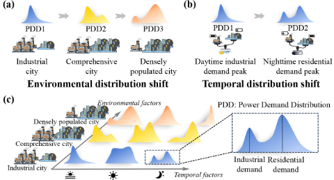
The growing complexity of dynamical systems has driven the demand for accurate and efficient simulation methods [Kumar et al., 2020; Cui et al., 2024]. However, traditional experience-driven numerical simulators are too ideal and computationally intensive, making it difficult to efficiently simulate complex scenarios. Due to the outstanding function approximation power from neural networks, neural simulators have successfully emerged, demonstrating excellent computability and accuracy in simulating various artificial and natural systems, such as the climate system influenced by human activities [Min et al., 2011], energy management system [R. Singh et al., 2024], and so on. By identify- Figure 1: (a) Distribution shift induced by environmental variations, where electricity demand differs significantly across cities due to variations in industrial activity, climate, or population density. (b) Distribution shift induced by temporal variations, where the patterns of use of electricity fluctuate throughout the day. (c) These two types of distribution shifts often occur together in practical applications. This dual presence of variations complicates to generalize across both environmental and temporal dimensions, necessitating a solution that adapt to both variations simultaneously.
∗Corresponding authors
ing key patterns in seemingly unpredictable evolutions, these simulators offer valuable insights into system behavior and long-term tendencies [Zhou et al., 2022] and facilitating more informed decision-making [Nouinou et al., 2023].
The current neural simulators are mainly based on recurrent neural networks (RNN) [Rajalingham et al., 2022; Barbulescu et al., 2023], neural differential equations [Chen et al., 2022; Laurie and Lu, 2023], and their combinations [Li et al., 2022]. These methods benefit from the strengths of neural networks in learning complex patterns and the continuity of differential equations in modeling dynamics to address concerns on complex temporal dependencies, irregular sampling, and high computational costs. However, most of them operate under the assumption that the data is independently and identically distributed (i.i.d.), where the observation of system state from distinct time steps and sequences is generated from a consistent distribution [Bai et al., 2023]. This assumption, while theoretically convenient, rarely holds in practical scenarios, which are inherently influenced by external factors beyond system boundary, including environmental and temporal variations, causing the tough distribution shift problem in the observed system, making the i.i.d. neural simulators ineffective.
Distribution shifts induced by environmental variations [Koh et al., 2021; Cui et al., 2024] arise when the observed sequences are derived from distinct environmental conditions. A clear example, as shown in Fig.1(a), is the power grid system, where electricity demand differs significantly across cities due to variations in industrial activity, climate, or population density. In industrialized cities, commercial electricity demand dominates, while in residential regions, household electricity demand plays a greater role [Yan et al., 2024]. Environmental variations challenge the neural simulators' ability to generalize across data distributions, limiting the capacity to inherit predictive accuracy when applied to system dynamics governed by different environmental conditions. To tackle this, several approaches strive to attempt to learn dynamical systems across diverse environments by using a shared component for common behaviors and an environment-specific component for unique variations, such as LEADS [Yin et al., 2021], CoDA [Kirchmeyer et al., 2022], and CoNDP [Liu et al., 2024].
On the other hand, when the observed system states evolve with time-sensitive external conditions, distribution shifts induced by temporal variations may occur [Koh et al., 2021], even under a consistent environmental setting. In the power grid system, the patterns of use of electricity fluctuate throughout the day: during daytime, commercial demand peaks as businesses operate, whereas at night, residential demand rises as households consume more electricity [Yan et al., 2024],, as shown in Fig. 1(b). These temporal shifts make it difficult for simulators to capture non-stationary dynamics, reducing its capacity to maintain predictive performance as the system's behavior evolves over time. To mitigate the impact of such shifts, recent neural simulators have begun to consider parameter dynamics [Bai et al., 2023; Liu et al., 2023; Cai et al., 2024], where the model parameters are dynamically changing over time, to enhance adaptability and efficiency.
Although existing advanced methods have made significant strides in addressing distribution shifts induced by environmental [Yin et al., 2021; Kirchmeyer et al., 2022; Liu et al., 2024] or temporal variations [Bai et al., 2023; Liu et al., 2023; Cai et al., 2024], there is a lack of a solution that can simultaneously consider addressing both aspects of distribution shifts. In practical applications, these two types of distribution shifts often occur together. We still take the common power system as an example: these shifts occur concurrently-electricity demand fluctuates both due to environmental factors (e.g., industrial v.s. residential areas) and temporal changes (e.g., day v.s. night).
To that end, we propose a novel neural simulator to model both environmental and temporal distribution shifts in a holistic framework. It innovatively represents the system's evolution as a stochastic process governed by a time-sensitive combination of basic differential equations, capturing both temporal distribution shifts, influenced by time-evolving environments, and the multi-phase transitions, thereby generalizing to new environments, sparsity, and noise.
The main contributions are summarized as follows:
- We propose a Context-informed Polymorphic Neural ODE Processes (CoPoNDP) to effectively address environmental and temporal distribution shifts. To our knowledge, this is the first work to tackle both shifts in neural simulators within a unified framework.
- The CoPoNDP can effectively handle sparsity and noise in dynamical systems by leveraging context-driven network modulation and uncertainty modeling, ensuring robustness even with incomplete or noisy data.
- Comprehensive experiments are performed on representative complex dynamical systems from ecology, chemistry, physics, and energy, showcasing its effectiveness with superior results compared to existing models.
2 RelatedWork and Problem Statement
2.1 RelatedWork
Neural Simulators under i.i.d. Assumption
Recent advancements in neural simulators have demonstrated their versatility in modeling complex dynamical systems across diverse fields, such as exploring the role of dynamic reasoning in primate behavior by comparing mental simulations with recurrent neural networks (RNN) [Rajalingham et al., 2022], predicting ultrashort pulse propagation in optical fibers through a long-short-term memory-based model [Salmela et al., 2021], and successfully simulating the locomotion behavior of C. elegans [Barbulescu et al., 2023].
As a novel class of deep learning models, neural differential equations can model continuous dynamics by parameterizing the derivative of hidden states using neural networks [Chen et al., 2018]. They have shown remarkable potential in predicting metabolomic profiles from microbial composition [Wang et al., 2023], forecasting outcomes in spintronic experiments [Chen et al., 2022], and modeling tumor dynamics for survival prediction [Laurie and Lu, 2023].
The current methods that combine RNN and neural differential equations enhance the ability to handle irregularly sampled data and capture complex temporal dependencies [Li et al., 2022]. Although the above studies emphasize the growing utility of neural simulators in capturing and predicting system dynamics from biological processes to physical phenomena, and their high computational efficiency compared to traditional experience-driven approaches, they still struggle with tasks that have non-i.i.d. characteristics and often appear in real world, resulting in good theoretical models but limited practical effects.
Environmental Adaptive Neural Simulators
To handle non-i.i.d. scenarios, several studies have been starting to explore learning dynamical systems across varying environments [Yin et al., 2021; Kirchmeyer et al., 2022; Liu et al., 2024]. As a pioneer in addressing multi-environment scenarios, LEADS models system dynamics with a shared component and an environment-specific component, and then freezes the shared component while tuning environmentspecific parameters for new environments [Yin et al., 2021].
CoDA employs a hypernetwork to generate environmentspecific parameters from learnable compact parameters, reducing parameter tuning and mitigating overfitting [Kirchmeyer et al., 2022]. In order to solve the problem of data sparsity caused by costly acquisition or sensor failures [Huang et al., 2020], CoNDP goes beyond the deterministic models mentioned above and incorporates uncertainty modeling in learning underlying dynamical systems [Liu et al., 2024]. It uses a context-informed encoder to produce a conditional distribution over environment representations and models dynamics with random control vectors, and this stochasticity enables it to better capture system evolution under data scarcity, improving generalization by learning from uncertainty in environmental factors [Liu et al., 2024].
Temporal Adaptive Neural Simulators
Temporal domain generalization (TDG) has emerged as a promising way to address the temporal distribution shift and non-stationary [Li et al., 2020a; Nasery et al., 2021; Qin et al., 2022; Bai et al., 2023; Yong et al., 2023; Zeng et al., 2024]. Traditional TDG methods, such as S-MLDG [Li et al., 2020a] and GI [Nasery et al., 2021], use discrete time steps to model temporal shifts, which can be limiting in capturing continuous dynamics. To enhance flexibility, DRAIN introduces a Bayesian framework that models the joint dynamics of data and model parameters [Bai et al., 2023], leveraging recurrent graph-based networks with learning temporal drift to predict future states. This approach provides theoretical guarantees on generalization error and uncertainty [Bai et al., 2023], though it is still constrained by its discretetime assumption. Koopa [Liu et al., 2023] and Koodos [Cai et al., 2024] offer innovative solutions for continuous-time dynamics modeling. Koopa introduces Koopman theory to tackle non-stationary time series [Liu et al., 2023], which employs Fourier filters and Koopman predictors to disentangle and model time-variant and time-invariant dynamics hierarchically, achieving competitive performance with improved efficiency and interpretability. Koodos also uses Koopman operators to linearize complex temporal dynamics and allows for predictions at arbitrary time points, facilitating generalization over irregular intervals [Cai et al., 2024].
2.2 Problem Statement
In this work, we focus on handling complex dynamical systems evolving under a time-varying environmental factor, whose evolution is governed by the following Ordinary Differential Equation (ODE):
where, xet ∈ Rdx represents the state of the system at time t under a time-varying environment e and uet = ge (t) ∈ Rdu corresponds to the time-varying environment e at time t, with ge (t) sampled from a Banach space. The dimensions of the system state and time-varying environmental factor are denoted by dx and du, respectively. Note that the indices e and t in uet characterize the impact of the environment and time on the dynamical system, where changes in e can cause the environmental distribution shift, while changes in t result in non-stationary dynamics with the temporal distribution shift.
Due to the wide and complex correlations, external factors are often difficult to accurately obtain [Kirchmeyer et al., 2022; Liu et al., 2024], resulting in uet not being disclosed. This requires the model to have the ability to represent and capture external changes and generalize learning directly from avaliable observed data. Formally, we define the observed system states within the environment e at certain time points, which are necessary information in predicting future states, as the context C e = {xeti : i ∈ I e C }, where I e C is the set of indexes of the time points. And, let the system states at time points that we aim to predict denote the target T e = {xetj : j ∈ I e T }, where I e T refers to the indexes of the time points for which predictions are made. Our goal is to learn a generalizable simulator S that learns to map from contexts to targets, approximating the underlying f with various time-varying environments, i.e.,
where E is the number of time-varying environments. Therefore, the learned S can predict the system states xe′ tj under a time-varying unseen environment e′ at any time tj∈I e′ T , based on the context C e′ , i.e., S(C e′ ) → T e′ . Note that the timestamps can exhibit non-uniform intervals and are allowed to take continuous values.
3 CoPoNDP: Context-Informed Polymorphic Neural ODE Processes
In this section, we introduce a context-informed polymorphic neural ODE processes (CoPoNDP) that is designed to handle both temporal and environmental distribution shifts in dynamical systems.
3.1 Model Overview
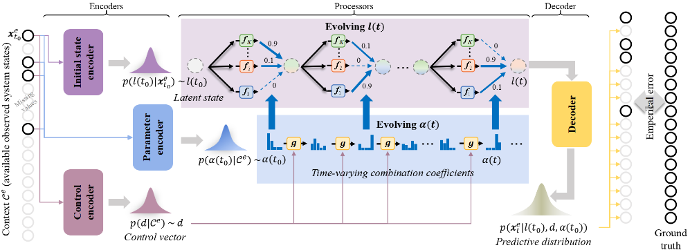
CoPoNDP is mainly implemented based on the sandwich architecture of encoders-processors-decoder, as shown in Fig. 2. Encoders generate several distributions based on the context C e as starting points for subsequent processing, including the distribution of initial latent states, i.e., p(l(t0)|xet0 ), distribution of initial time-varying combination coefficients, i.e., p(α(t0)|C e ), and distribution of global control vector, i.e., p(d|C e ). Processors are to evolve the latent state l(t) and combination coefficients α(t) respectively, starting from the sampling of generated distributions, accounting for both temporal dynamics and environmental variation. Decoder can restore the evolved latent state l(t) to the space of system states and output the predictive distribution on environment e at any time t, i.e., p(xet |l(t0), d, α(t0)).
3.2 Encoders
Encoders are responsible for generating distributions of initial latent states, combination coefficients, and control vector.
Initial State Encoder: Given the initial observation xet0 at time t0, the initial state encoder encφl generates a Gaussian distribution of the initial latent state, i.e., p(l(t0)|xet0 ) = N (µl , σ2 l ). The mean and variance of the distribution are obtained from
where φl denotes the learnable parameters that are updated during the training phase. The initial latent state l(t0) determines the starting point for dynamic evolution in hidden space. Note that lt0 is a random vector so that it can generate diverse starting points in prediction.
Parameter Encoder: Given the context C e , the parameter encoder encφα can produce a Gaussian distribution of the initial time-varying combination coefficients, i.e., p(α(t0)|C e ) = N(µα, σ2α), whose mean and variance are determined by
where φα are the learnable parameters. The initial combination coefficients α(t0) can serve as an uncertain starting point for the evolution of the time-varying α(t).
Control Encoder: Given the environmental context C e , a Gaussian distribution of the random control vector, i.e., p(d|C e ) = N (µd, σ2 d ), can be generated by
where encφd is the control encoder and φd is its learnable parameters. Note that the random control vector d encodes the context-dependent information, capturing environmental conditions and past system states, which directly affects how the model evolves over time, ensuring that variations brought about by environmental changes are effectively integrated.
3.3 Processors
Processors evolve the latent states l(t) and the time-varying combination coefficients α(t).
Evolution on the Latent State l(t): We model a continuous process to evolve the latent states. Specifically, we assume that the continuous and complex evolution can be composed of a weighted combination of K orthogonal differential equations, i.e., f1, f2, ..., fK, which has flexible and sufficient expressive power across environments. For these basic differential equations, we use neural ODEs [Chen et al., 2018] to model separately. That is to say, l(t) = ∑Kk=1 αk(t) × lk(t), where αk(t) is the time-varying coefficients, whose evolution will be introduced later, and each branch lk(t) is evolved as
where l(t0) ∼ p(l(t0)|xet0 ).
Evolution on the Time-Varying Coefficients α(t): The evolution process of α(t) = [α1(t); ...; αK(t)] ∈ RK can be formulated as
where α(t0) ∼ p(α(t0)|C e ) and d ∼ p(d|C e ). g is a neural ODE that can govern how the importance of different components in the latent state changes over time. Before combining αk(t) and lk(t), it is necessary to perform a softmax operation to keep the sum of the combination coefficients at 1. It is worth emphasizing here that the time-varying coefficients can ensure adaptation to temporal distribution shift. In the coefficient evolution process, the control vector d also participates as an input, which enables the model to adaptively control its evolution based on context from different environments.
3.4 Decoder
Using the evolved latent states l(t) and placing a Gaussian distribution on system states, we can obtain the predictive system states at any time t by employing a decoder as
where, decφx is the decoder, φd is its learnable parameters, and µx and σ2x are the mean and variance of the predictive distribution, i.e., p(xet |l(t0), d, α(t0)) = N(µx, σ2x ), which can accommodate system noise.
3.5 Training and Adapating
New, we introduce the overall training procedure of the CoPoNDP. We randomly generate E time-varying environments for a dynamical system by sampling g1 (t), g2 (t), ... from a Banach space, and obtain sparse trajectories through irregularly sampling observations under each environment. Then, we divide these trajectories into two halves, where the first half is contexts, i.e., {C e}Ee=1 , and the second half is targets, i.e., {T e}Ee=1 . Based on the contexts and targets, we jointly train all parts in an end-to-end fashion to achieve a generalizable simulator. Specifically, following [Liu et al., 2024], we use the variational inference to train the neural networks in the model, i.e., encφl , encφα , encφd , f1, ..., fK, g, and decφx , whose specific architectures can be found in supplementary material. 1 . The variational lower bound to be maximized can be formulated as
where qlt0 ,d,αt0 = p(l(t0)|xet0 )p(d|C e )p(α(t0)|C e ). When adapting to a new time-varying environment e′ , by inputting the available observations C e′ , we can obtain the predictive distribution at any time t, i.e., p(xe′ t |l(t0), d, α(t0)).
3.6 CoPoNDP as Stochastic Process
From a probabilistic perspective, our CoPoNDP can actually be seen as a type of neural-network-parameterized stochastic process for system states.
Proposition 1. CoPoNDP satisfies the exchangeability and consistency conditions.
The detailed proof can be found in supplementary material. According to the Kolmogorov Extension Theorem, we know that exchangeability and consistency conditions are sufficient to define a stochastic process [Oksendal, 2013]. That is to say, the stochastic processes we have established exist, and the CoPoNDP is its family of finite-dimensional distributions. As a stochastic process, it should theoretically have the ability to represent dynamical systems with a wide range of time-varying environments, and also can have excellent generalization power for sparse and noisy settings.
4 Experiment
We test the CoPoNDP 2 on four representative complex dynamical systems in various fields to answer the following questions: 1) How well does our model generalize to simultaneous environmental and temporal distribution shifts by learning from observed contexts? 2) What factors in our model impact performance? 3) How does the level of sparsity and noise in the context affect the model's adaptation to distribution shifts? 4) Can our model adapt to distribution shifts appearing in real-time streaming data?
1 https://github.com/ljqjlu/CoPoNDP/blob/main/supp-
2 Our code is available at https://github.com/ljqjlu/CoPoNDP.
4.1 Experiment Settings
We are here to introduce experiment settings, including dynamical systems, baselines, and task descriptions. For a detailed introduction to dynamical systems and the experimental setup, please refer to the supplementary materials.
Dynamical Systems. We conducted a series of experiments to thoroughly evaluate the model's capabilities and its applicability to real-world scenarios, focusing on a wide range of systems affected by time-sensitive external conditions, including the pendulum with external control forces (PE) [Baker and Blackburn, 2008], the ecosystem with timevarying birth and death rates (LV) [Wangersky, 1978], the controlled vibration of a string fixed at both ends (ST) [Wang and Wang, 2013], and the real-world datasets such as power system demand forecasting (PW) [Zhou et al., 2021], exchange prediction (EX) [Lai et al., 2018], air quality (AQ) [Zhang et al., 2017] and weather forecasting (WT) [Han et al., 2024].
Baselines. We compare our CoPoNDP against twelve state-of-the-art neural simulators for dynamical systems, which can be divided into four main groups. 1) Neural simulators under i.i.d. assumption include the discrete models, i.e., GRU [Cho et al., 2014] and LSTM [Hochreiter, 1997], and continuous models, i.e., Neural ODE [Chen et al., 2018] and ODE-RNN [Chen et al., 2018]. 2) Environmental adaptive neural simulators contain the LEADS [Yin et al., 2021], CoDA [Kirchmeyer et al., 2022], and CoNDP [Liu et al., 2024]. 3) Temporal adaptive neural simulators contain the DRAIN [Bai et al., 2023], Koopa [Liu et al., 2023], Koodos [Cai et al., 2024], and Koopman-DG [Zeng et al., 2024]. 4) We also compare recently emerging neural operators, including the Fourier Neural Operator (FNO) [Li et al., 2020b], Factorized Fourier Neural Operator (FFNO) [Tran et al., 2021], Geometry-Aware Fourier Neural Operator (Geo-FNO) [Li et al., 2023], general neural operator transformer (GNOT) [Hao et al., 2023] and the Deep Operator Network (DeepONet) [Lu et al., 2021], to verify the simultaneous processing of two types of distribution shifts. However, unlike our model, the neural operators require a known time-varying environment of the task to be processed as input.
Task Descriptions. We set up four testing tasks to evaluate the impact of varying degrees of distribution shifts on model generalization. In-Distribution Test: uet in Eq. 1 remains identical and constant throughout training and testing, unchanged by time or environment, indicating stable and consistent conditions. Environmental Adaptation (Env. Ada.) Test: uet differs between training and testing but remains constant over time, testing adaptability to new environments without temporal shifts. Temporal Adaptation (Tem. Ada.) Test: uet is the same for training and testing but varies over time, focusing on adaptation to dynamic temporal changes.
| In-Distribution | Env. Ada. Test | Tem. Ada. | Test | Joint-Distribution | Real-World Datasets | ||||||||||||
|---|---|---|---|---|---|---|---|---|---|---|---|---|---|---|---|---|---|
| Models | PE (×10-6 ) | LV (×10-5 ) | ST (×10-4 ) | PE (×10-5 ) | LV (×10-4 ) | ST (×10-4 ) | PE (×10-5 ) | LV (×10-4 ) | ST (×10-4 ) | PE (×10-5 ) | LV (×10-4 ) | ST (×10-4 | PW ) (×100 ) | EX (×10-4 | AQ ) (×100 ) | WT (×100 ) | |
| GRU | 3.42 | 5.15 | 2.91 | 1.52 | 2.14 | 8.84 | 1.42 | 5.63 | 8.92 | 11.23 | 13.49 | 13.81 | 11.2 | 2.03 | 153.40 | 3.81 | |
| i.i.d. Ass. LSTM | 2.97 | 4.83 | 3.11 | 1.68 | 1.92 | 8.27 | 2.13 | 4.58 | 8.37 | 11.34 | 14.05 | 14.93 | 12.5 | 2.14 | 142.64 | 4.39 | |
| Neural ODE | 4.08 | 6.20 | 3.55 | 1.33 | 1.58 | 8.43 | 3.47 | 6.19 | 9.04 | 11.48 | 13.88 | 13.13 | 13.3 | 2.20 | 123.61 | 3.45 | |
| ODE-RNN | 3.78 | 5.35 | 3.29 | 1.42 | 1.54 | 9.63 | 1.68 | 5.13 | 8.27 | 9.19 | 13.22 | 14.58 | 10.4 | 2.09 | 116.87 | 3.58 | |
| LEADS | 2.59 | 4.21 | 3.11 | 0.217 | 0.241 | 3.39 | 1.29 | 4.56 | 6.84 | 8.35 | 10.13 | 9.52 | 1.388 | 1.28 | 7.22 | 1.49 | |
| Env. Ada. CoDA | 2.32 | 4.83 | 3.59 | 0.295 | 0.223 | 4.01 | 1.72 | 5.11 | 7.03 | 9.46 | 9.98 | 9.29 | 1.416 | 1.06 | 7.53 | 1.57 | |
| CoNDP | 2.01 | 4.49 | 4.12 | 0.203 | 0.258 | 4.16 | 1.94 | 5.37 | 6.45 | 11.59 | 12.22 | 8.87 | 2.372 | 1.10 | 6.47 | 1.34 | |
| DRAIN | 1.79 | 3.92 | 2.87 | 1.18 | 1.47 | 7.32 | 0.143 | 0.408 | 3.22 | 11.09 | 9.25 | 9.24 | 0.351 | 0.318 | 5.25 | 0.333 | |
| Tem. Ada. Koopa | 1.11 | 4.21 | 3.15 | 1.45 | 1.69 | 7.57 | 0.138 | 0.443 | 2.94 | 11.28 | 10.37 | 9.63 | 0.301 | 0.323 | 4.97 | 0.330 | |
| Koodos | 1.47 | 4.67 | 3.61 | 1.59 | 1.83 | 6.71 | 0.206 | 0.505 | 3.53 | 10.32 | 11.61 | 8.97 | 0.333 | 0.301 | 5.12 | 0.327 | |
| Koopman-DG | 1.38 | 4.19 | 3.02 | 1.04 | 1.31 | 6.49 | 0.142 | 0.415 | 3.30 | 9.28 | 9.61 | 9.34 | 0.333 | 0.294 | 4.93 | 0.315 | |
| CoPoNDP (Ours) | 1.23 | 4.18 | 3.08 | 0.196 | 0.214 | 3.29 | 0.132 | 0.377 | 3.14 | 0.176 | 0.420 | 3.21 | 0.277 | 0.275 | 4.49 | 0.287 | |
Joint-Distribution Test: uet varies both between training and testing and over time, evaluating model generalization to simultaneous environmental and temporal shifts. Although the PW is not modeled by differential equations, it still aligns with the Joint-Distribution Test, because it is simultaneously influenced by external environmental factors (cities, weather) and temporal factors (periodic human activities). For each task, we sample extensive time-varying environments for testing and then compare the average performance.
4.2 Performance Evaluation
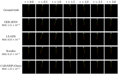
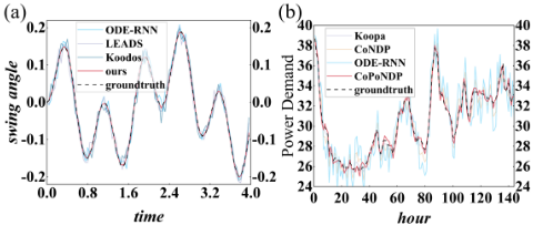
From Table 1, we see that under the In-Distribution Test, our CoPoNDP has comparable performance, providing relatively stable predictions and confirming its reliability under minimum distribution shifts. Under the Environmental Adaptation Test, compared to i.i.d. models and temporal adaptive neural simulators, environmental adaptive models, such as LEADS, CoDA, and CoNDP, perform well with a reduction in error of almost an order of magnitude. The better performance of the temporal adaptive models is under the Temporal Adaptation Test. And, our CoPoNDP achieves the best performance in both settings mentioned above, demonstrating its effectiveness in handling unilateral distribution shifts. In the Joint-Distribution Test, the CoPoNDP significantly outperforms others, reducing error by order of magnitude for the PE and LV systems. The pendulum visualizations of the PE system are shown in Figs. 3 and 4(a). For the ST system and real-world PW data, our CoPoNDP also achieves the best results, showcasing the generalization of our model for the simultaneous occurrence of environmental and temporal distribution shifts. Please see Fig. 4(b) for the comparison of the actual electricity demand forecast results.
We also compare our CoPoNDP with neural operators, as shown in Table 2. Even though operator-based models are highly effective, they require a known time-varying environment as input, which restricts their practicality. In contrast, our CoPoNDP can learn system dynamics influenced by distribution shifts from only observed system states. This eliminates the need for environmental input and allows it to achieve state-of-the-art results compared to other models with the same level of information, while effectively generalizing to practical applications.
4.3 Ablation Study and Sensitivity Analysis
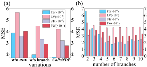
To analyze the rationality behind our model, we conducted two variants of the CoPoNDP. One variant involved our model without the control encoder, denoted as w/o control encoder, to verify the role of context in model evolution. The other was our model without multiple basic neural differential equations, and only one differential equation was used for modeling, i.e., w/o branches, to test the expressive power of the combination of basic equations for distribution shifts. From Fig. 5(a), we see that our model outperforms these variants across all systems under the existence of two distribution shifts, showcasing the effectiveness of the model design. The setting of the number of basic neural differential equations (branches) seriously affects the model's expressive power for dealing with external time-varying environmental changes. To analyze the impact of the number of branches, we tested configurations ranging from 2 to 10 neural differential equations, as shown in Fig. 5(b). Initially, model performance improved as the number of branches increased, reaching its peak at 5 to 6 branches. Beyond this range, the performance benefits plateaued, and in some instances, adding more branches slightly decreased performance due to over-parameterization and increased computational overhead. These findings suggest a need for balance between model flexibility and efficiency in selecting the number of equation branches.
| Models | w/ env. state | w/o env. state | ||
|---|---|---|---|---|
| PE (×10-6 ) | LV (×10-5 | PE ) (×10-6 ) | LV (×10-5 ) | |
| FNO | 0.234 | 0.713 | 7.67 | 7.34 |
| FFNO | 0.187 | 0.695 | 6.30 | 5.41 |
| Operators Geo-FNO | 0.249 | 0.3548 | 2.37 | 5.83 |
| GNOT | 0.154 | 0.388 | 3.29 | 6.33 |
| DeepONet | 0.416 | 0.884 | 4.69 | 6.57 |
| CoPoNDP (Ours) | - | - | 1.76 | 4.20 |
4.4 Generalization to Sparse and Noisy Data
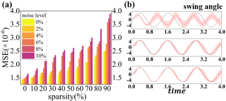
To assess the robustness of CoPoNDP, we expanded our analysis to include sparse and noisy conditions under joint distribution shifts on the PE system. This involved incorporating different levels of data sparsity, ranging from 0% to 90%, as well as Gaussian noise levels from 0% to 10% in the observed contexts. Fig. 6(a) shows that although the model prediction error slightly increases with higher sparsity and noise intensity, the decline in our model's performance is limited and negligible compared to an error of 83.5×10⁻⁶ from the best baseline, i.e., LEADS, under 50% sparsity and noisefree observations. This demonstrates our CoPoNDP's resilience, even when the observed context is highly fragmented or noisy. The above results also suggest that perfect contextual knowledge is not a strict requirement for effective adaptation. Instead, CoPoNDP can capture sufficient uncertainty through its probabilistic structure, which integrates context into both context encoding and latent process evolution.
4.5 Contextual Adaptation to Streaming Data
Since the principle behind our CoPoNDP is a stochastic process, it not only brings more heightened tolerance for sparsity and noise but also inherits the data adaptation from the stochastic process. As more input data are provided, the CoPoNDP can adaptively correct its predictions without retraining, essentially suitable for online processing of streaming data. We test its predictive accuracy by gradually increasing the amount of input data, as shown in Fig. 6(b). This setup mirrors real-world conditions, where systems must adjust to evolving data distributions without full context availability at the outset. We can see that as the amount of contextual data increases, the model adapts and adjusts to obtain predictions that are closer to the true values, with decreasing uncertainty. The initial increments, especially the addition of the first 3% of context, led to the most substantial performance improvements. As more context was added, accuracy continued to increase, eventually reaching a saturation point at 5% data. This demonstrates the system's effectiveness in adapting to partial, real-time data streams. The observation highlights its adaptation to external changes, driven by progressively refining its understanding as new context is provided, ensuring reliable performance in time-varying dynamical systems.
5 Conclusion
We introduce CoPoNDP, a neural ODE framework that models dynamical systems under temporal and environmental distribution shifts by dynamically blending context-aware ODE ensembles. Unlike existing simulators limited to static or single-axis adaptation, CoPoNDP achieves robust generalization across ecological, chemical and physical systems, outperforming specialized baselines.
While demonstrating strong empirical performance, scaling to real-world applications requires further advances in automated architecture optimization and physics-aware efficiency improvements. Our work establishes an important step toward generalizable neural simulators that adapt to complex, evolving dynamics while maintaining computational tractability.
Acknowledgments
This work was supported by the National Key R&D Program of China (Grant No. 2021ZD0112500), National Natural Science Foundation of China (Grant Nos. U22A2098, 62172185, 62206105 and 62202200), Natural Science Foundation of Jilin Province (Grant No. 20250102211JC), Scientific Research Project of Education Department of Jilin Province (Grant No. JJKH20250118KJ), and Jilin Province Youth Science and Technology Talent Support Project (Grant No. QT202225).
@inproceedings{ijcai2025p841,
  title     = {Towards Generalizable Neural Simulators: Addressing Distribution Shifts Induced by Environmental and Temporal Variations},
  author    = {Liu, Jiaqi and Cui, Jiaxu and Sun, Shiang and Zhao, Yizhu and Yang, Bo},
  booktitle = {Proceedings of the Thirty-Fourth International Joint Conference on
               Artificial Intelligence, {IJCAI-25}},
  publisher = {International Joint Conferences on Artificial Intelligence Organization},
  editor    = {James Kwok},
  pages     = {7563--7571},
  year      = {2025},
  month     = {8},
  note      = {Main Track},
  doi       = {10.24963/ijcai.2025/841},
  url       = {https://doi.org/10.24963/ijcai.2025/841},
}
TY - CPAPER TI - Towards Generalizable Neural Simulators: Addressing Distribution Shifts Induced by Environmental and Temporal Variations AU - Liu, Jiaqi AU - Cui, Jiaxu AU - Sun, Shiang AU - Zhao, Yizhu AU - Yang, Bo T2 - Proceedings of the Thirty-Fourth International Joint Conference on Artificial Intelligence, IJCAI-25 PB - International Joint Conferences on Artificial Intelligence Organization PY - 2025 SP - 7563 EP - 7571 DO - 10.24963/ijcai.2025/841 UR - https://doi.org/10.24963/ijcai.2025/841 ER -Copied
Machine-readable versions of this paper, for tools and AI agents:





