
StreamMTS: Towards Streaming Multivariate Time Series Forecasting
Proceedings of the Thirty-Fifth International Joint Conference on Artificial Intelligence. Main Track. Pages 3061-3069.
https://doi.org/10.24963/ijcai.2026/340
Keywords
- Data Mining: Mining spatial and/or temporal data
Abstract
Current mainstream research in multivariate time series (MTS) forecasting often assumes that all data are static. However, real-world MTS data typically arrives continuously in a streaming manner, which we refer to as streaming MTS. The statistical characteristics and spatiotemporal graph topology of these data evolve over time, presenting two key challenges: the model's ability to adapt to new data distributions and the enhancement of cross-domain generalization capabilities. In this paper, we propose a streaming MTS prediction framework. We begin by designing a lightweight spatiotemporal causal learning model that captures generalizable causal spatiotemporal features from a decoupling perspective. Next, we introduce a framework to enhance the model's streaming learning capability, leveraging the adaptability of continual learning while strengthening cross-domain representation abilities. Specifically, we reformulate continual learning as a multi-task learning problem and present a multi-task optimization algorithm that identifies a set of Pareto-optimal solutions to address the inherent stability-plasticity dilemma in continual learning. Finally, we propose a topology-aware feature propagation strategy that disseminates well-trained node embedding features to unseen graph structures, thereby improving the model's cross-domain generalization. Results on real-world datasets demonstrate that our model achieves superior forecasting performance while substantially improving computational efficiency and memory usage.
- [An et al., 2025] Rui An, Yifeng Zhang, Ziran Liang, Wenqi Fan, Yuxuan Liang, Xuequn Shang, and Qing Li. Damba- st: Domain-adaptive mamba for efficient urban spatio- temporal prediction. arXiv preprint arXiv:2506.18939, 2025.
- [Chen and Liang, 2024] Wei Chen and Yuxuan Liang. Ex- pand and compress: Exploring tuning principles for con- tinual spatio-temporal graph forecasting. arXiv preprint arXiv:2410.12593, 2024.
- [Chen et al., 2021] Xu Chen, Junshan Wang, and Kunqing Xie. Trafficstream: A streaming traffic flow forecasting framework based on graph neural networks and continual learning. arXiv preprint arXiv:2106.06273, 2021. IJCAI
- [Cirstea et al., 2021] Razvan-Gabriel Cirstea, Tung Kieu, Chenjuan Guo, Bin Yang, and Sinno Jialin Pan. En- hancenet: Plugin neural networks for enhancing corre- lated time series forecasting. In 2021 IEEE 37th Inter- national Conference on Data Engineering (ICDE), pages 1739-1750. IEEE, 2021.
- [Deng et al., 2021] Jinliang Deng, Xiusi Chen, Renhe Jiang, Xuan Song, and Ivor W Tsang. St-norm: Spatial and tem- poral normalization for multi-variate time series forecast- ing. In Proceedings of the 27th ACM SIGKDD conference on knowledge discovery & data mining, pages 269-278, 2021.
- [Désidéri, 2012] Jean-Antoine Désidéri. Multiple-gradient descent algorithm (mgda) for multiobjective optimization. Comptes Rendus Mathematique, 350(5-6):313-318, 2012.
- [Fang et al., 2023] Yuchen Fang, Yanjun Qin, Haiyong Luo, Fang Zhao, Bingbing Xu, Liang Zeng, and Chenxing Wang. When spatio-temporal meet wavelets: Disentan- gled traffic forecasting via efficient spectral graph attention networks. In 2023 IEEE 39th International Conference on Data Engineering (ICDE), pages 517-529. IEEE, 2023.
- [Gong et al., 2020] Yongshun Gong, Zhibin Li, Jian Zhang, Wei Liu, and Yu Zheng. Online spatio-temporal crowd flow distribution prediction for complex metro system. IEEE Transactions on knowledge and data engineering, 34(2):865-880, 2020.
- [Hamilton et al., 2017] Will Hamilton, Zhitao Ying, and Jure Leskovec. Inductive representation learning on large graphs. Advances in neural information processing sys- tems, 30, 2017.
- [Jiang et al., 2023] Jiawei Jiang, Chengkai Han, Wayne Xin Zhao, and Jingyuan Wang. Pdformer: Propagation delay- aware dynamic long-range transformer for traffic flow pre- diction. arXiv preprint arXiv:2301.07945, 2023.
- [Jin et al., 2023] Guangyin Jin, Yuxuan Liang, Yuchen Fang, Zezhi Shao, Jincai Huang, Junbo Zhang, and Yu Zheng. Spatio-temporal graph neural networks for predictive learning in urban computing: A survey. IEEE Transac- tions on Knowledge and Data Engineering, 2023.
- [Kieu et al., 2024] Duc Kieu, Tung Kieu, Peng Han, Bin Yang, Christian S Jensen, and Bac Le. Team: Topo- logical evolution-aware framework for traffic forecasting- extended version. arXiv preprint arXiv:2410.19192, 2024.
- [Kirkpatrick et al., 2017] James Kirkpatrick, Razvan Pas- canu, Neil Rabinowitz, Joel Veness, Guillaume Des- jardins, Andrei A Rusu, Kieran Milan, John Quan, Tiago Ramalho, Agnieszka Grabska-Barwinska, et al. Overcom- ing catastrophic forgetting in neural networks. Proceed- ings of the national academy of sciences, 114(13):3521- 3526, 2017.
- [Lee and Park, 2024] Sanghyun Lee and Chanyoung Park. Continual traffic forecasting via mixture of experts. arXiv preprint arXiv:2406.03140, 2024.
- [Lin et al., 2019] Xi Lin, Hui-Ling Zhen, Zhenhua Li, Qing- Fu Zhang, and Sam Kwong. Pareto multi-task learning. Advances in neural information processing systems, 32, 2019.
- [Liu et al., 2023] Hangchen Liu, Zheng Dong, Renhe Jiang, Jiewen Deng, Jinliang Deng, Quanjun Chen, and Xuan Song. Spatio-temporal adaptive embedding makes vanilla transformer sota for traffic forecasting. In Proceedings of the 32nd ACM international conference on information and knowledge management, pages 4125-4129, 2023.
- [Liu et al., 2025a] Jiayue Liu, Zhongchao Yi, Zhengyang Zhou, Qihe Huang, Kuo Yang, Xu Wang, and Yang Wang. Synevo: A neuro-inspired spatiotemporal evo- lutional framework for cross-domain adaptation. arXiv preprint arXiv:2505.16080, 2025.
- [Liu et al., 2025b] Zhanyu Liu, Guanjie Zheng, and Yanwei Yu. Multi-scale traffic pattern bank for cross-city few-shot traffic forecasting. ACM Transactions on Knowledge Dis- covery from Data, 19(4):1-24, 2025.
- [Liu et al., 2025c] Zhipeng Liu, Peibo Duan, Xuan Tang, Baixin Li, Yongsheng Huang, Mingyang Geng, Chang- sheng Zhang, Bin Zhang, and Binwu Wang. Time- former: Transformer with attention modulation empow- ered by temporal characteristics for time series forecast- ing. Expert Systems with Applications, page 131040, 2025.
- [Ma et al., 2025a] Jiaming Ma, Binwu Wang, Pengkun Wang, Zhengyang Zhou, Xu Wang, and Yang Wang. Bist: A lightweight and efficient bi-directional model for spa- tiotemporal prediction. Proceedings of the VLDB Endow- ment, 18(6):1663-1676, 2025.
- [Ma et al., 2025b] Jiaming Ma, Binwu Wang, Pengkun Wang, Zhengyang Zhou, Xu Wang, and Yang Wang. Ro- bust spatio-temporal centralized interaction for ood learn- ing. In Forty-second International Conference on Machine Learning, 2025.
- [Pareja et al., 2020] Aldo Pareja, Giacomo Domeniconi, Jie Chen, Tengfei Ma, Toyotaro Suzumura, Hiroki Kaneza- shi, Tim Kaler, Tao Schardl, and Charles Leiserson. Evolvegcn: Evolving graph convolutional networks for dynamic graphs. In Proceedings of the AAAI conference on artificial intelligence, volume 34, pages 5363-5370, 2020.
- [Sener and Koltun, 2018] Ozan Sener and Vladlen Koltun. Multi-task learning as multi-objective optimization. Ad- vances in neural information processing systems, 31, 2018.
- [Shao et al., 2022a] Zezhi Shao, Zhao Zhang, Fei Wang, Wei Wei, and Yongjun Xu. Spatial-temporal identity: A simple yet effective baseline for multivariate time series forecast- ing. In Proceedings of the 31st ACM International Con- ference on Information & Knowledge Management, pages 4454-4458, 2022.
- [Shao et al., 2022b] Zezhi Shao, Zhao Zhang, Wei Wei, Fei Wang, Yongjun Xu, Xin Cao, and Christian S Jensen. De- coupled dynamic spatial-temporal graph neural network for traffic forecasting. arXiv preprint arXiv:2206.09112, 2022.
- [Sun et al., 2024] Yuan Sun, Shang Li, Li Fu, Lu Yin, and Zhongliang Deng. Nicl: Non-line-of-sight identification in global navigation satellite systems with continual learning. IEEE Transactions on Vehicular Technology, 2024.
- [Wang et al., 2020] Shuo Wang, Yanran Li, Jiang Zhang, Qingye Meng, Lingwei Meng, and Fei Gao. Pm2. 5-gnn: A domain knowledge enhanced graph neural network for pm2. 5 forecasting. In Proceedings of the 28th interna- tional conference on advances in geographic information systems, pages 163-166, 2020.
- [Wang et al., 2023a] Binwu Wang, Yudong Zhang, Jiahao Shi, Pengkun Wang, Xu Wang, Lei Bai, and Yang Wang. Knowledge expansion and consolidation for continual traf- fic prediction with expanding graphs. IEEE Transactions on Intelligent Transportation Systems, 24(7):7190-7201, 2023.
- [Wang et al., 2023b] Binwu Wang, Yudong Zhang, Xu Wang, Pengkun Wang, Zhengyang Zhou, Lei Bai, and Yang Wang. Pattern expansion and consolidation on evolving graphs for continual traffic prediction. In Proceedings of the 29th ACM SIGKDD Conference on Knowledge Discovery and Data Mining, pages 2223-2232, 2023.
- [Wang et al., 2024] Binwu Wang, Pengkun Wang, Yudong Zhang, Xu Wang, Zhengyang Zhou, Lei Bai, and Yang Wang. Towards dynamic spatial-temporal graph learning: A decoupled perspective. In Proceedings of the AAAI Con- ference on Artificial Intelligence, volume 38, pages 9089- 9097, 2024.
- [Wu et al., 2019] Zonghan Wu, Shirui Pan, Guodong Long, Jing Jiang, and Chengqi Zhang. Graph wavenet for deep spatial-temporal graph modeling. arXiv preprint arXiv:1906.00121, 2019. IJCAI
- [Xia et al., 2023] Yutong Xia, Yuxuan Liang, Haomin Wen, Xu Liu, Kun Wang, Zhengyang Zhou, and Roger Zim- mermann. Deciphering spatio-temporal graph forecast- ing: A causal lens and treatment. arXiv preprint arXiv:2309.13378, 2023.
- [Yan et al., 2025] Han Yan, Dongliang Chen, Guiyuan Jiang, Bin Wang, Lei Cao, Junyu Dong, and Yanwei Yu. Dgraformer: Dynamic graph learning guided multi-scale transformer for multivariate time series forecasting. In Proceedings of the Thirty-Fourth International Joint Con- ference on Artificial Intelligence (IJCAI 2025), pages 3516-3524, 2025. IJCAI
- [Yang et al., 2021] Song Yang, Jiamou Liu, and Kaiqi Zhao. Space meets time: Local spacetime neural network for traffic flow forecasting. In 2021 IEEE International Con- ference on Data Mining (ICDM), pages 817-826. IEEE, 2021.
- [Yu et al., 2017] Bing Yu, Haoteng Yin, and Zhanxing Zhu. Spatio-temporal graph convolutional networks: A deep learning framework for traffic forecasting. arXiv preprint arXiv:1709.04875, 2017. IJCAI
- [Yuan et al., 2024] Yuan Yuan, Jingtao Ding, Jie Feng, De- peng Jin, and Yong Li. Unist: a prompt-empowered uni- versal model for urban spatio-temporal prediction. In Pro- ceedings of the 30th ACM SIGKDD Conference on Knowl- edge Discovery and Data Mining, pages 4095-4106, 2024.
- Zeng et al., ] Hanqing Zeng, Hongkuan Zhou, Ajitesh Sri- vastava, Rajgopal Kannan, and Viktor Prasanna. Graph- saint: Graph sampling based inductive learning method. In International Conference on Learning Representations.
- [Zeng et al., 2023] Ailing Zeng, Muxi Chen, Lei Zhang, and Qiang Xu. Are transformers effective for time series fore- casting? In Proceedings of the AAAI conference on artifi- cial intelligence, volume 37, pages 11121-11128, 2023.
- [Zhang et al., 2019] Zhengchao Zhang, Meng Li, Xi Lin, Yinhai Wang, and Fang He. Multistep speed prediction on traffic networks: A deep learning approach considering spatio-temporal dependencies. Transportation research part C: emerging technologies, 105:297-322, 2019.
- [Zhang et al., 2025] Haoyu Zhang, Wentao Zhang, Hao Miao, Xinke Jiang, Yuchen Fang, and Yifan Zhang. Strap: Spatio-temporal pattern retrieval for out-of-distribution generalization. arXiv preprint arXiv:2505.19547, 2025.
- [Zhao et al., 2024] Zhe Zhao, Pengkun Wang, Haibin Wen, Yudong Zhang, Zhengyang Zhou, and Yang Wang. A twist for graph classification: Optimizing causal informa- tion flow in graph neural networks. In Proceedings of the AAAI Conference on Artificial Intelligence, volume 38, pages 17042-17050, 2024.
- [Zheng et al., 2024] Jialun Zheng, Divya Saxena, Jiannong Cao, Hanchen Yang, and Penghui Ruan. Inductive spa- tial temporal prediction under data drift with informative graph neural network. In International Conference on Database Systems for Advanced Applications, pages 169- 185. Springer, 2024.
References were extracted automatically from the PDF and may contain errors.
Full text extracted automatically from the PDF; figures, tables and equations may differ. The PDF is the version of record.
1 Introduction
Spatiotemporal graph neural networks (STGNN) [An et al., 2025; Jin et al., 2023; Ma et al., 2025a] have become the most popular tool for multivariate time series (MTS) prediction. Despite achieving impressive performance, STGNNs primarily excel in static scenarios where MTS data characteristics and underlying graph topology remain stable. However, in practical applications, MTS data is typically collected continuously in a streaming manner, referred to as streaming MTS. A key characteristic of streaming MTS is its nonstationarity: on the one hand, the statistical features and joint distribution of MTS exhibit variability; on the other hand, the scale of graph topology, which reflects the number of variables in MTS, changes over time [Zhang et al., 2025; Liu et al., 2025a]. Notably, in many application systems, graph topology tends to expand globally in the long term. For example, modern cities frequently expand their transportation networks to accommodate population growth, introducing new sensors. Additionally, some countries are increasingly focusing on air quality, incorporating new monitoring devices into atmospheric quality monitoring systems.
∗Yudong Zhang and Yang Wang are the corresponding authors.
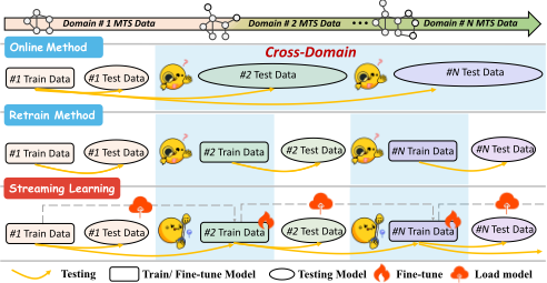
To achieve streaming MTS prediction, a simple online learning approach involves transferring models trained in the initial domain for prediction in subsequent domains without additional fine-tuning processes. However, this strategy fails to effectively incorporate new knowledge from subsequent domains 1 , resulting in poor performance. Another approach is the retraining method, which involves training a new model for each domain. However, this method raises concerns about high computational complexity. An efficient alternative is continual learning, which continues the training process using data from new domains while overcoming catastrophic forgetting [Wang et al., 2023b; Chen et al., 2021].
1 To incorporate streaming MTS into our research problem, we divide it into different domains, where data features remain relatively stable within domains while varying between domains.
However, as illustrated in Figure 1, both retraining and continual learning methods rely on the assumption that adequate training data has been collected beforehand, prior to starting the training or fine-tuning process for each domain. Once training is complete, models are evaluated using data from the same domain. Challenges arise during crossdomain phases, where the features of the data for training the model do not align with the test data, often involving the data collection phase for new domains. Due to limited crossdomain generalization capabilities, these models find it difficult to perform zero-shot prediction tasks on cross-domain MTS data that diverges from the training distribution. In this context, the streaming learning framework highlights the dual objectives of continuous learning and generalization: continuously integrating new knowledge while reducing catastrophic forgetting within each domain and ensuring robust cross-domain generalization abilities. We encounter the following challenges:
- How to absorb new knowledge and consolidate old knowledge. Key studies in continual spatiotemporal learning, such as TrafficStream [Chen et al., 2021] and PECMP [Wang et al., 2023b], face a common challenge known as the plasticity-stability dilemma. Model stability aims to limit the updates of weights to retain previously acquired knowledge. This approach is beneficial when the features of the current domain align closely with those of earlier domains, as it helps reinforce prior learning. However, when the features diverge, it becomes essential to prioritize model plasticity, enabling significant weight adjustments for the swift integration of new concepts. Consequently, a more nuanced strategy is required to foster a flexible continual learning process.
2. How to improve the model's cross-domain generalization. Existing STGNNs struggle to adapt to diverse testing environments due to their reliance on the training features of MTS. Specifically, GCNs utilize message-passing mechanisms along the edges of trained graphs to generate graph representations. This approach often results in learned parameters that do not generalize effectively to unseen graph topologies [Hamilton et al., 2017; Zeng et al., ]. Additionally, the parameters of some SOTA STGNNs, such as D2STGNN, are closely tied to the scale of the graph topology. Consequently, when the graph topology changes during cross-domain, these STGNNs fail to perform prediction testing on the evolved graph. Moreover, GCNs rely on knowledge learned from existing graph topology to generate rough representations for new nodes through message mechanisms. However, these representations can be biased and contain significant noise, leading to a decline in the overall accuracy of the graph.
This paper proposes a streaming MTS prediction framework (StreamMTS) 2 . Specifically, we first introduce a lightweight spatiotemporal causal learning model to capture causal knowledge from streaming spatiotemporal data from a decoupled perspective, where this knowledge maintains consistent dynamics in streaming data. Then, we design a streaming framework to enable this model to perform streaming prediction. This framework inherits continual learning's adaptability to streaming data while enhancing the model's representation capability during the cross-domain phase. In detail, we first formulate continual learning as a Pareto multi-task problem, then introduce a multi-objective optimization algorithm that decomposes the multi-task into a set of constrained subproblems with different trade-off preferences. This algorithm can find a set of representative Pareto-optimal solutions with different trade-offs between stability and plasticity. Furthermore, to enhance the model's representation capability during the cross-domain phase, we design a topology-aware feature propagation strategy. This strategy generates beneficial node representations for new nodes by diffusing welltrained node embeddings. Our contributions are as follows:
2 https://github.com/ContinualGoing/IJCAI STREAMMTS
- We introduce a pioneering problem: streaming MTS prediction, which extends static MTS analysis to a more practical scenario.
- We design a streaming MTS prediction framework that incorporates a lightweight spatiotemporal causal learning model and a cross-domain enhanced Pareto continual learning strategy.
- Extensive experiments demonstrate that our model achieves superior forecasting performance while substantially improving computational efficiency and memory usage.
2 ProblemDefinition
Multivariate Time Series (MTS). Let X ∈ RL×N denote the MTS data from N variables with L time steps. We use xt ∈ RN to denote the MTS data at time step t. We represent MTS data as a graph G = {V, A, E}, where V represents N nodes (i.e., variables) in the graph. E means the set of edges and A ∈ RN×N is the adjacency matrix of the graph G to describe the node connections.
Streaming MTS. Multivariate time series are collected in a streaming manner. We partition the SMTS data into distinct domains, wherein data distributions evolve and graph topological structures expand over time 3 . Specifically, we use G = {G 1 , · · · , G τ , · · · } and X = {X1 , · · · ,Xτ , · · · } to represent streaming MTS data, where G τ = {V τ ,Aτ , E τ }, and Xτ represents the MTS data in the τ -th domain. Given i < j, we have N i < N j and the data distribution P(Xi ) ̸= P(Xj ). Streaming MTS Prediction. Given SMTS data X with G, the goal of SMTS prediction is to sequentially train a streaming prediction model F, and in the τ-th domain, Fτ takes the input X ∈ RT×N = {xt-T+1, · · · , xt} from past T time steps, which is sampled from the current domain Xτ or crossdomain Xτ+1 , to effectively predict the MTS data for the next Tp time steps, Y = {xt+1, · · · , xt+Tp }.
3 Method
In this section, we present the details of our proposed StreamMTS, which consists of two key components: a spatiotemporal causal learning model and a streaming learning framework that enables this spatiotemporal learning model to perform streaming MTS prediction. The pseudo-code is obtained in algorithm 1.
3 We assume that the graph topology remains stable within each domain.
3.1 Spatiotemporal LearningModel
Given that GCN or Transformers exhibit high complexity, limited generalization, and poor scalability when modeling spatial dependencies for new nodes in streaming MTS, we propose a simple MLP-based spatiotemporal learning model. Additionally, to enhance the model's ability to capture spatiotemporal dynamics, we incorporate embedding techniques to encode various prior knowledge.
Following prior works [Yuan et al., 2024; Shao et al., 2022a], we employ embedding techniques to encode prior information to enhance the model's representation capability. We encode the day-of-week and timestep-of-day information into the model, and utilize node embedding techniques to capture the semantic features of each node. We utilize a learnable embedding vector Et ∈ RNt×de to encode the information of each time step within a day, where Nt represents the number of data points in a day. For instance, with a sampling frequency of five minutes, a day would comprise 288 data points, thus setting Nt to 288. We also adopt a learnable embedding vector E d τ ∈ RNd×de to encode day of week information, where Nd represents the number of days in a week and is equal to 7. We further develop a learnable node embedding vector Esτ ∈ RNτ×de to represent the features of Nτ nodes in the graph. We concatenate these embeddings and the input, which is defined as H0τ .
Then we use L layers of MLP with a residual connection to model the spatiotemporal dynamics of H0τ . Specifically, the l-th MLP layer can be denoted as:
where σ means activation function, here, we use RELU activation. Hlτ means the input of l-th layer, when l=0, the input is H0τ . After L MLP layers, the output is denoted as the nonstationary components ZNon τ . Next, we use a reverse residual technology to decouple the causal knowledge, which is denoted as:
Then we obtain stationary caucal components by removing non-stationary components ZNon τ :
Finally, the causal components are inputted into the decoder composed of an MLP layer to generate stationary predictions, allowing the model to more easily handle nonstationary MTS. Similarly, we also incorporate the nonstationary components into the output. The process can be defined as:
We minimize the L1 loss between predicted value ˆYτ and ground-truth value Yτ :
where Lp means the regression loss.
3.2 Pareto Spatiotemporal Continual Learning
To enable the spatiotemporal learning model to perform streaming MTS prediction, the continual learning paradigm is gaining momentum. This paradigm involves sequentially training models using time series data from different domains to adapt to new data distributions. Among these approaches, regularization-based methods have achieved impressive performance by imposing additional constraints on model updates, with their optimization objective expressed as:
where Lr represents the regularization term, and λ is a hyperparameter that balances the two loss terms. θ denotes the parameters of the model.
In this paper, we employ Elastic Weight Consolidation (EWC) [Kirkpatrick et al., 2017], a representative method that utilizes the Fisher matrix to approximate the importance of parameters, and the updates of important parameters are limited to prevent catastrophic forgetting [Wang et al., 2023a; Sun et al., 2024]. Specifically, given the trained model Fτ in the τ-th domain, we first compute the Fisher information Ω to measure the importance of each parameter, and the importance of i-th parameter can be computed using first-order derivatives of the loss:
where Lp represents the regression loss. Then, the regularization loss in the continual learning process can be denoted as:
where Fτ (θi) denotes the value of the i-th parameter of Fτ . Finally, in the continual learning phase (i.e., τ > 0), our total loss function is:
where λ is a hyperparameter that balances two loss terms. θ means the parameters of the model.
In fact, λ regulates the model's plasticity towards old knowledge and its scalability towards new knowledge. When λ is large, model updates are severely restricted, causing the model to favor consolidating old knowledge while limiting its ability to absorb new knowledge. Conversely, when λ is small, the model tends to absorb new knowledge but compromises its plasticity towards old knowledge. In the context of continual learning, selecting an appropriate λ in equation 9 can be highly challenging. To address this issue, we creatively formulate continuous learning as a multi-objective optimization problem and introduce the Pareto multi-task approach as a solution [Lin et al., 2019].
Pareto Multi-Task Learning
In the real world, many problems involve optimizing multiple objectives simultaneously. Multi-Objective Optimization Algorithms have been developed to address these challenges.
These algorithms aim to identify solutions that optimize multiple objectives, resulting in a set of solutions that offer various trade-offs, known as the Pareto optimal solution set.
If a task problem involves a set of m correlated loss functions with a loss vector:
where Lm(θ) means the value of m-th loss function. Multiobjective optimization problems are usually solved with the goal of achieving overall optimality (Pareto optimality) [D´esid´eri, 2012; Zhao et al., 2024], which provides the optimal trade-offs among all loss targets. It is worth noting that such optimal solutions are not unique. In this paper, we aim to find a set of well-distributed Pareto solutions that can represent different trade-offs between two loss targets (i.e., M=2). Next, we explain some important definitions.
Definition 1. (Pareto dominance). A solution θ1 dominates a solution θ2 if and only if Li (θ1 ) ≤ Li (θ2 ) , ∀i ∈ {1, . . . ,M}, and L (θ1 ) ̸= L (θ2 ).
Definition 2. (Pareto optimality). A solution θ is considered Pareto optimal if there is no other solution θ∗ that dominates it. This means that θ∗ is not inferior to any other solution with respect to all objectives.
Definition 3. (Pareto Set and Pareto Front). The Pareto Set, Θ∗ , is the set of all Pareto optimal solutions, defined as Θ∗ (θ < Θ | θ∗ ⊂ Θ such that θ∗ < θ). The Pareto Front, L(Θ∗ ), is the image of the Pareto Set in the objective space, defined as L(Θ∗ ) = {L(θ) | θ ∈ Θ∗ }.
We employ the Pareto Multi-Task Learning algorithm (Pareto MTL) [Lin et al., 2019], which decomposes the multi-objective optimization problem into multiple subproblems with multiple constraints. First, we find a set of welldistributed unit preference vectors {u1, u2, . . . , uK} in RM + , where K means the number of subspaces. For the preference vector uK, the multi-objective sub-problem is defined as:
where Ωk (k = 1, ..., K) is a sub-region in an objective space and with u⊤j v is the inner product between the preference vector uj and a given vector v:
If a vector v belongs to Ωk, it means that v has the smallest acute angle with the vector uk and, consequently, the largest inner product u⊤k v among all K preference vectors.
The preference vectors serve to partition the objective space into distinct sub-regions, where the potential solutions within each sub-region embody varying trade-offs between the two tasks at hand. To tackle these multi-objective subproblems effectively, a two-step, gradient-based method is employed for solution optimization.
To solve the constrained multi-objective subproblem described in Equation 11, we reformulate this problem as unconstrained optimization, and use a sequential gradient-based method to find the initial solution θ0.
Specifically, following a methodology akin to prior studies [Sener and Koltun, 2018; Lin et al., 2019], the problem is reformulated into an unconstrained optimization problem. This transformation aims to employ an efficient descent direction that effectively mitigates all active constraints within the optimization process.
where dt is the search direction, which is used as the descent direction for the constrained MOO. α is the constraint of direction. I (θr) = {j | Gj (θr) ≥ 0, j = 1, . . . ,K} is denoted as the index set of all activated constraints, and {Gj (θr) | j ∈ I (θr)} means all activated constraints.
Due to the high dimensionality of the problem, we transform the decision space from the parameter space to a more manageable objective and constraint space; for the proof of transforming the decision space from the parameter space to a more manageable objective and constraint space, please refer to the work [Lin et al., 2019]. This allows Pareto MTL to be extended and optimized for our task, as shown in Equation 9. The output of Pareto MTL is a set of allocation weights (α1 and α2) to balance two tasks in Equation 9. Finally, the balancing factor λ equals (α2/α1).
Topology-Aware Feature Propagation Strategy
During the cross-domain phase, the model Fτ trained in τth domain needs to make prediction on new spatiotemporal graph signals X ∈ RT×Nτ+1 . The main challenge is to improve the representation capability for newly added nodes, as these nodes are unseen to the model. To address this challenge, we propose feature propagation strategies.
During training, our spatiotemporal model's parameterized learnable node embeddings Esτ ∈ RNτ×de capture high-level features for Nτ nodes from the data. Considering that connected nodes in a graph share similar features, we aim to transfer these information-rich node embeddings to generate effective node embeddings for newly added nodes.
Specifically, we use the normal distribution random initialization strategy to initialize an embedding, which is denoted as Epτ ∈ R∆Nτ×de , for ∆Nτ new nodes, where ∆Nτ = Nτ+1 -Nτ . And Epτ is expected to be smooth on the graph such that nearby nodes have similar node embedding. Generally, the solution can be approximated via the iteration as follows:
where Z denotes the number of power iteration (propagation) steps. The transition matrix T ∈ R∆Nτ×Nτ indicates the dependency of the newly added node and the original node and is a part of the normalized adjacency matrix. After Z iterations of feature propagation, the predicted embedding feature matrix Epτ is capable of capturing the prior knowledge of the neighborhood feature distribution up to Z hops away.
During the fine-tuning in the τ-th domain, Esτ is concatenated with the node embeddings to form an expanded node embedding, which is updated to accurately capture the semantic features of the new nodes.
Algorithm 1 StreamMTS for streaming MTS prediction
Input: Testing data Xτ s and training data Xτ+1 t
Parameter: Trained model at τ -th domain Fτ
Output: Trained model Fτ+1
- 1: ## Testing in the τ-th domain.
- 2: Testing Fτ using testing data Xτ s .
- 3: ## Testing in the cross-domain.
- 4: Epτ ←Esτ according to Equation 14.
- 6: TestingFτ withEsτ using the training dataXτ+1 t in τ +1th domain.
- 5: Esτ ← [Epτ ,Epτ ].
- 7: ## Continual learning in the (τ +1)-th domain.
- 8: Finetue Fτ with Esτ using the training data Xτ+1 t .
- 9: return solution
4 Experiment
4.1 Dataset
We utilize two streaming MTS datasets, namely PEMS3Stream and Air-Stream. PEMS3-Stream [Chen et al., 2021], derived from traffic flow data, consists of seven temporal domains, each spanning a month with a sampling frequency of five minutes. The number of nodes in this dataset ranges from 655 to 871. Air-Stream dataset is generated by KnowAir [Wang et al., 2020] and contains up to 186 nodes. It is divided into 12 time domains, each of which lasts for one month. The details of these two datasets are shown in Table 1. We provide a more detailed explanation in the Appendix.
| Dataset | PEMS3-Stream | Air-Stream |
| Nodes Sampling frequency Domains Field | 655→871 5 minutes 7 Traffic | 78→184 1 hour 12 Atmosphere |
4.2 Baseline
For compared baselines that include retraining methods and continuous learning methods, we split the data from each domain into training, validation, and testing sets in a ratio of 6:2:2 along the time axis. During the cross-domain period, we continue to perform prediction tasks using the trained baselines until the training pipeline accumulates training sets from the subsequent domain.
1. Retraining Methods include the following advanced models: STGCN [Yu et al., 2017], GWNet [Wu et al., 2019], DCRNN [Deng et al., 2021], STAEformer [Liu et al., 2023], STNN [Yang et al., 2021], STWave [Fang et al., 2023], EvolveGCN [Pareja et al., 2020], EnhanceNet [Cirstea et al., 2021], and DLinear [Zeng et al., 2023]. For some models, we need to make necessary modifications to non-core code to adapt to a streaming setting.
- Continuous Learning Methods include: TrafficStream [Chen et al., 2021], STKEC [Wang et al., 2023a],
- PECPM [Wang et al., 2023b], Expand-SurST [Chen et al., 2021], INF-GNN [Zheng et al., 2024], EAC [Chen and Liang, 2024], and TFMoE [Lee and Park, 2024].
- Online Learning Methods include: STONE [Wang et al., 2024] and CaST [Xia et al., 2023]. For the online learning strategy, we train their model with the first domain data and then test directly on the next domains.
4.3 Setting
We set both the input and prediction windows to 12 in traffic prediction and 24 in atmospheric prediction. We implement all models using PyTorch framework of Python 3.8.3 and leveraging the Nvidia A100-PCIE-40GB as support, and adopt Adam optimizer with a learning rate of 0.002. MAE, RMSE, and MAPE are used as metrics for comparison. We set the maximum batch size to 100 with early stopping strategy to prevent overfitting. α and Z are set to 0.2 and 2 respectively. The embedding feature dimension de is set to 32.
4.4 Prediction Performance Comparison
Streaming MTS Prediction Comparison
The experimental results on the PEMS3-Stream dataset are shown in Table 3. We report the average test performance within and across domains. We can observe that retraining methods generally perform better than continual learning approaches. This is because these continual learning algorithms use only a subset of the new domain's training set to continue the training process, primarily to improve training efficiency. However, this subset cannot cover all new knowledge, leading to suboptimal performance.
Specifically, regarding retraining methods, GWNet performs well, thanks to its comprehensive modeling of multigranular temporal dependencies. Overall, retraining methods underperform compared to our model. On one hand, training a new model for each new domain fails to effectively utilize previously learned knowledge. On the other hand, their insufficient cross-domain prediction capability leads to poor performance. As for online training strategies, these methods focus on extracting invariant knowledge from different training environments to improve generalization. However, they cannot timely absorb new knowledge, resulting in inadequate performance. Our framework achieves good prediction performance because we inherit the ability of continuous learning to model the dynamics of streaming data and also improve the cross-domain prediction performance of the model.
| Model | MAE | RMSE | MAPE |
|---|---|---|---|
| TrafficStream | 16.37 | 27.04 | 22.94 |
| PECPM | 14.76 | 25.03 | 18.30 |
| TFMoE | 14.18 | 23.54 | 18.36 |
| INF-GNN | 16.83 | 27.47 | 26.45 |
| ECA | 13.53 | 21.77 | 18.98 |
| Ours | 11.10 | 19.01 | 15.13 |
| 3-step | 6-step | 12-step | ||||||||
|---|---|---|---|---|---|---|---|---|---|---|
| Model | MAE | RMSE | MAPE | MAE | RMSE | MAPE | MAE | RMSE | MAPE | |
| GWNet | 12.03 | 19.90 | 15.84 | 13.17 | 21.91 | 17.59 | 15.64 | 25.61 | 20.17 | |
| STGCN | 12.55 | 20.74 | 17.92 | 13.72 | 22.77 | 19.12 | 16.17 | 26.81 | 22.26 | |
| STWave | 12.54 | 21.29 | 18.18 | 13.96 | 23.86 | 20.07 | 16.06 | 27.46 | 23.02 | |
| TrendGCN | 13.11 | 21.83 | 17.58 | 14.45 | 23.93 | 19.41 | 18.14 | 32.80 | 26.19 | |
| Retrain | EvolveGCN | 14.50 | 23.96 | 20.70 | 15.85 | 26.30 | 22.08 | 18.68 | 30.97 | 25.71 |
| EnhanceNet | 14.43 | 23.85 | 20.60 | 15.78 | 26.18 | 21.98 | 18.59 | 30.83 | 25.59 | |
| DCRNN | 12.80 | 21.15 | 18.28 | 13.99 | 23.23 | 19.50 | 16.49 | 27.35 | 22.71 | |
| DLinear | 15.74 | 24.73 | 21.63 | 17.04 | 26.94 | 23.13 | 19.72 | 31.37 | 25.38 | |
| STAEformer | 12.35 | 19.78 | 15.64 | 13.21 | 22.41 | 17.82 | 15.62 | 26.39 | 19.91 | |
| Continual | TrafficStream | 14.04 | 22.68 | 21.48 | 16.11 | 26.32 | 24.41 | 21.41 | 34.62 | 33.14 |
| STKEC | 14.18 | 22.91 | 20.70 | 16.08 | 26.59 | 23.46 | 21.63 | 34.98 | 31.48 | |
| PECPM | 13.42 | 21.06 | 19.85 | 15.65 | 23.28 | 21.59 | 18.94 | 30.62 | 24.31 | |
| Expand-SurST | 15.19 | 24.57 | 22.56 | 18.12 | 29.69 | 25.67 | 24.76 | 40.47 | 33.86 | |
| Online | STONE | 13.27 | 21.48 | 17.06 | 14.30 | 23.68 | 18.23 | 16.28 | 28.41 | 20.94 |
| CaST | 15.43 | 24.53 | 32.15 | 17.13 | 27.63 | 33.77 | 20.96 | 33.82 | 39.07 | |
| Streaming | Ours | 11.05 | 18.63 | 14.99 | 11.84 | 20.22 | 16.19 | 13.37 | 22.92 | 18.53 |
Continual MTS Prediction Comparison
Since some advanced continual spatiotemporal models have not been open-sourced, we aligned with their experimental settings to reproduce their reported performance for a comprehensive comparison. Unlike streaming MTS prediction, continual MTS prediction focuses solely on withindomain continual prediction tasks, neglecting the crossdomain phase. The results are presented in Table 2.
We can find that our model achieved optimal performance. This is because these continual MTS prediction models use a subset of the training set to fine-tune the model. These subsets cannot comprehensively represent new knowledge, resulting in the model's inability to properly fit new data distributions, thus reducing prediction accuracy. Our model, which relies on a causal spatiotemporal graph learning model, can effectively learn generalizable knowledge. Additionally, benefiting from the Pareto MTL learning strategy, our model achieves better plasticity and stability, maintaining superior continual learning capability in streaming data.
| Model | MAE | RMSE | MAPE |
|---|---|---|---|
| GWNet | 14.41 | 23.47 | 19.03 |
| STGCN | 14.70 | 23.65 | 19.64 |
| STWave | 16.73 | 29.03 | 25.98 |
| DCRNN | 16.78 | 27.42 | 22.42 |
| STAEformer | 16.23 | 24.91 | 21.59 |
| PECPM | 18.24 | 29.04 | 24.08 |
| DLinear | 17.68 | 28.12 | 25.45 |
| Ours | 12.95 | 22.00 | 17.88 |
4.5 Cross-domain Performance Comparison
We specifically reported the cross-domain prediction performance of several advanced models on the PEMS3-Stream dataset. As shown in Table 4, we can observe that our model achieves optimal cross-domain performance. For spatiotemporal graph convolutional networks, while they can rely on GCN to generalize learned knowledge to newly added nodes, this representation is inaccurate as GCN's generalization ability to unknown graphs is limited. The Transformer-based model, STAEformer, shows poor cross-domain performance because Transformers struggle to extend learned knowledge to new nodes. Our model, however, achieves superior crossdomain performance, thanks to the causal spatiotemporal learning model that can capture invariant knowledge, which is beneficial for generating representations for newly added nodes. Additionally, we employed a topology-aware feature propagation strategy to enhance the representation capability of newly added nodes.
4.6 Efficiency Comparison
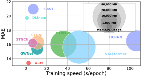
We compared the efficiency of several state-of-the-art models. We report the model memory usage (under optimal results) and training time per epoch, as shown in Figure 2. We found that our model achieved dominant performance in both training time and memory usage. Compared to STAEformer, we achieve over 10× improvement in speed and memory efficiency. This is because our model is based on an MLP architecture, and owing to several design choices, our model achieved high prediction accuracy.
4.7 Ablation Experiment
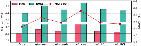
We evaluate the effectiveness of each component in our proposed method by creating the following variants: (1) w/o nemb represents removing node embeddings; (2) w/o temb represents removing temporal embeddings; (3) w/o cau indicates using fully connected layers for spatiotemporal learning while removing the causal learning structure; (4) w/o tfp represents removing the topology-aware feature propagation strategy; (5) w/o PCL indicates removing the Pareto multitask learning strategy. The results are shown in Figure 3.
w/o nemb achieved poor performance because node embeddings can capture high-level features from the data; w/o tfp resulted in larger prediction errors since this strategy enables effective generalization to new nodes by transferring learned knowledge, thereby enhancing representational capacity. Overall, all components of our model are effective.
4.8 Performance Comparison on Air-Stream
We evaluated model effectiveness on another dataset, AirStream. We set the input and prediction windows to 24, and reported prediction performance for 6, 12, and 24 time steps. The performance shown in Table 5 indicates that STAEformer performs poorly because it requires large amounts of data to fit spatiotemporal features. STGCN achieves good prediction performance because its lightweight model architecture can quickly learn spatiotemporal patterns. Our model remains effective, with performance improvements averaging over 5%.
5 RelatedWork
Spatiotemporal Prediction Recently, advances in deep learning have motivated the development of spatiotemporal graph neural networks to capture complex spatial and temporal dependencies in multivariate time series data [Ma et al., 2025a; Liu et al., 2025c; Ma et al., 2025b; Gong et al., 2020;
| 6-step | 12-step | 24-step | ||||
|---|---|---|---|---|---|---|
| KnowAir | MAE | RMSE | MAE | RMSE | MAE | RMSE |
| GWNet | 12.36 | 16.55 | 13.82 | 18.12 | 14.41 | 18.78 |
| STGCN | 11.72 | 15.65 | 11.47 | 15.60 | 11.80 | 16.02 |
| STWave | 12.19 | 15.99 | 12.49 | 16.90 | 13.16 | 16.98 |
| STAEformer | 14.28 | 17.49 | 14.68 | 20.35 | 16.26 | 21.07 |
| DCRNN | 13.26 | 16.44 | 14.23 | 17.25 | 14.55 | 18.01 |
| DLinear | 13.78 | 17.49 | 13.72 | 17.64 | 14.72 | 17.25 |
| Ours | 10.80 | 15.36 | 11.24 | 16.10 | 11.49 | 16.75 |
Yan et al., 2025; Liu et al., 2025b]. Representative models such as D2STGNN [Shao et al., 2022b] and PDFormer [Jiang et al., 2023] incorporate Transformer to model spatiotemporal dynamics more effectively. Although these approaches have demonstrated empirical performance across a range of applications, they are primarily designed for static settings in which data distributions and graph structures remain stable over time. In contrast, real-world systems often collect multivariate time series data in a streaming manner, where both temporal patterns and underlying graph topologies evolve. Existing retraining and online learning strategies for extending spatiotemporal graph neural networks to streaming scenarios struggle to cope with such non-stationarity, limiting their adaptability in dynamic environments.
Spatiotemporal Continual Prediction Researchers [Chen and Liang, 2024; Zheng et al., 2024] introduced continual learning strategies to achieve dynamic MTS learning. Most representative works [Chen et al., 2021; Wang et al., 2023a; Wang et al., 2023b; Kieu et al., 2024] proposed subgraph sampling strategies, where a subgraph is sampled during each continual learning process to fine-tune the model. This subgraph is expected to contain new temporal features and neighborhood relationships. For example, TrafficStream [Chen et al., 2021], PECPM [Wang et al., 2023b], and TEAM [Kieu et al., 2024] first evaluate each node's evolution degree between two consecutive domains, and sample representative nodes with both stable and unknown data distributions respectively. Although the subgraph sampling strategy demonstrates impressive computational efficiency by using only a portion of the entire graph, these subgraphs often fail to adequately cover the comprehensive information available in the complete graph, limiting GCN's ability to learn complete neighborhood relationships of the expanded graph.
6 Conclusion
We introduce a streaming multivariate time series prediction framework. It features a causal spatiotemporal learning model designed to capture robust spatiotemporal dynamics from a decoupling perspective. Additionally, we propose a streaming learning strategy that enables this model to perform streaming MTS predictions. This strategy leverages the adaptability of continual learning to dynamic data, while also enhancing cross-domain prediction capabilities. Extensive experiments validate the effectiveness of our model.
Acknowledgements
This work was partially supported by the National Natural Science Foundation of China (No.12227901) and the Natural Science Foundation of Jiangsu Province (BK20250482). The AI-driven experiments, simulations and model training were performed on the robotic AI-Scientist platform of Chinese Academy of Science.
@inproceedings{ijcai2026p340,
  title     = {StreamMTS: Towards Streaming Multivariate Time Series Forecasting},
  author    = {Wang, Binwu and Ma, Jiaming and Zhang, Yudong and Wang, Pengkun and Zhou, Zhengyang and Wang, Xu and Wang, Yang},
  booktitle = {Proceedings of the Thirty-Fifth International Joint Conference on
               Artificial Intelligence, {IJCAI-26}},
  publisher = {International Joint Conferences on Artificial Intelligence Organization},
  editor    = {Diego Calvanese},
  pages     = {3061--3069},
  year      = {2026},
  month     = {8},
  note      = {Main Track},
  doi       = {10.24963/ijcai.2026/340},
  url       = {https://doi.org/10.24963/ijcai.2026/340},
}
TY - CPAPER TI - StreamMTS: Towards Streaming Multivariate Time Series Forecasting AU - Wang, Binwu AU - Ma, Jiaming AU - Zhang, Yudong AU - Wang, Pengkun AU - Zhou, Zhengyang AU - Wang, Xu AU - Wang, Yang T2 - Proceedings of the Thirty-Fifth International Joint Conference on Artificial Intelligence, IJCAI-26 PB - International Joint Conferences on Artificial Intelligence Organization PY - 2026 SP - 3061 EP - 3069 DO - 10.24963/ijcai.2026/340 UR - https://doi.org/10.24963/ijcai.2026/340 ER -Copied
Machine-readable versions of this paper, for tools and AI agents:





