
DGraFormer: Dynamic Graph Learning Guided Multi-Scale Transformer for Multivariate Time Series Forecasting
Proceedings of the Thirty-Fourth International Joint Conference on Artificial Intelligence. Main Track. Pages 3516-3524.
https://doi.org/10.24963/ijcai.2025/391
Keywords
- Data Mining: DM: Mining spatial and/or temporal data
- Machine Learning: ML: Time series and data streams
Abstract
Multivariate time series forecasting is a critical focus across many fields. Existing transformer-based models have overlooked the explicit modeling of inter-variable correlations. Similarly, the graph-based methods have also failed to address the dynamic nature of multivariate correlations and the noise in correlation modeling. To overcome these challenges, we propose a novel Dynamic Graph Learning Guided Multi-Scale Transformer (DGraFormer) for multivariate time series forecasting. Specifically, our method consists of two main components: Dynamic correlation-aware graph Learning (DCGL) and multi-scale temporal transformer (MTT). The former aims to capture dynamic correlations across different time windows, filters out noise, and selects key weights to guide the aggregation of relevant feature representations. The latter can effectively extract temporal patterns from patch data at varying scales. Finally, the proposed method can capture rich local correlation graph structures and multi-scale global temporal features. Experimental results demonstrate that DGraformer significantly outperforms existing state-of-the-art models on ten real-world datasets, achieving the best performance across multiple evaluation metrics. The source code of our model is available at \url{https://anonymous.4open.science/r/DGraFormer}.
- [Abu-El-Haija et al., 2019] Sami Abu-El-Haija, Bryan Per- ozzi, Amol Kapoor, Nazanin Alipourfard, Kristina Ler- man, Hrayr Harutyunyan, Greg Ver Steeg, and Aram Gal- styan. Mixhop: Higher-order graph convolutional archi- tectures via sparsified neighborhood mixing. In ICML, pages 21-29, 2019.
- [Bai et al., 2018] Shaojie Bai, J Zico Kolter, and Vladlen Koltun. An empirical evaluation of generic convolutional and recurrent networks for sequence modeling. arXiv, 2018.
- [Brown et al., 2020] Tom Brown, Benjamin Mann, Nick Ry- der, Melanie Subbiah, Jared D Kaplan, Prafulla Dhari- wal, Arvind Neelakantan, Pranav Shyam, Girish Sastry, Amanda Askell, et al. Language models are few-shot learners. NeurlPS, 33:1877-1901, 2020.
- [Cai et al., 2024] Wanlin Cai, Yuxuan Liang, Xianggen Liu, Jianshuai Feng, and Yuankai Wu. Msgnet: Learning multi- scale inter-series correlations for multivariate time series forecasting. In AAAI, volume 38, pages 11141-11149, 2024.
- [Cao et al., 2025] Lingxiao Cao, Bin Wang, Guiyuan Jiang, Yanwei Yu, and Junyu Dong. Spatiotemporal-aware trend- seasonality decomposition network for traffic flow fore- casting. In AAAI, volume 39, pages 11463-11471, 2025.
- [Cao, 2022] Longbing Cao. Ai in finance: challenges, techniques, and opportunities. ACM Computing Surveys (CSUR), 55(3):1-38, 2022.
- [Chang et al., 2024] Zhiyong Chang, Mingjun Yin, and Yan Wang. Coatformer: vision transformer with composite at- tention. In IJCAI, pages 614-622, 2024. IJCAI
- [Chen et al., 2021] Zipeng Chen, Qianli Ma, and Zhenxi Lin. Time-aware multi-scale rnns for time series modeling. In IJCAI, pages 2285-2291, 2021. IJCAI
- [Chen et al., 2023] Ling Chen, Donghui Chen, Zongjiang Shang, Binqing Wu, Cen Zheng, Bo Wen, and Wei Zhang. Multi-scale adaptive graph neural network for multivari- ate time series forecasting. IEEE TKDE, 35(10):10748- 10761, 2023.
- [Chen et al., 2024] Peng Chen, Yingying Zhang, Yunyao Cheng, Yang Shu, Yihang Wang, Qingsong Wen, Bin Yang, and Chenjuan Guo. Pathformer: Multi-scale trans- formers with adaptive pathways for time series forecast- ing. In ICLR, 2024.
- [Das et al., 2023] Abhimanyu Das, Weihao Kong, Andrew Leach, Shaan Mathur, Rajat Sen, and Rose Yu. Long-term forecasting with tide: Time-series dense encoder. arXiv, 2023.
- [Defferrard et al., 2016] Michaël Defferrard, Xavier Bres- son, and Pierre Vandergheynst. Convolutional neural networks on graphs with fast localized spectral filtering. NeurlPS, 29, 2016.
- [Deng et al., 2022] Jinliang Deng, Xiusi Chen, Renhe Jiang, Xuan Song, and Ivor W Tsang. A multi-view multi-task learning framework for multi-variate time series forecast- ing. IEEE TKDE, 35(8):7665-7680, 2022.
- [Deng et al., 2024a] Jinliang Deng, Xiusi Chen, Renhe Jiang, Du Yin, Yi Yang, Xuan Song, and Ivor W Tsang. Disentangling structured components: Towards adaptive, interpretable and scalable time series forecasting. IEEE TKDE, 2024.
- [Deng et al., 2024b] Jinliang Deng, Feiyang Ye, Du Yin, Xuan Song, Ivor Tsang, and Hui Xiong. Parsimony or capability? decomposition delivers both in long-term time series forecasting. NeurlPS, 37:66687-66712, 2024.
- [Jiang et al., 2023] Jiawei Jiang, Chengkai Han, Wayne Xin Zhao, and Jingyuan Wang. Pdformer: Propagation delay- aware dynamic long-range transformer for traffic flow pre- diction. In AAAI, volume 37, pages 4365-4373, 2023.
- [Karita et al., 2019] Shigeki Karita, Nanxin Chen, Tomoki Hayashi, Takaaki Hori, Hirofumi Inaguma, Ziyan Jiang, Masao Someki, Nelson Enrique Yalta Soplin, Ryuichi Ya- mamoto, Xiaofei Wang, et al. A comparative study on transformer vs rnn in speech applications. In ASRU, pages 449-456. IEEE, 2019.
- [Kipf and Welling, 2016] Thomas N Kipf and Max Welling. Semi-supervised classification with graph convolutional networks. arXiv, 2016.
- [Kitaev et al., 2020] Nikita Kitaev, Lukasz Kaiser, and Anselm Levskaya. Reformer: The efficient transformer. In ICLR, 2020.
- [Lai et al., 2023] Zhichen Lai, Dalin Zhang, Huan Li, Chris- tian S Jensen, Hua Lu, and Yan Zhao. Lightcts: A lightweight framework for correlated time series forecast- ing. SIGMOD, 1(2):1-26, 2023.
- [Li et al., 2017] Yaguang Li, Rose Yu, Cyrus Shahabi, and Yan Liu. Diffusion convolutional recurrent neural net- work: Data-driven traffic forecasting. arXiv, 2017.
- [Li et al., 2023] Yiduo Li, Shiyi Qi, Zhe Li, Zhongwen Rao, Lujia Pan, and Zenglin Xu. Smartformer: Semi- autoregressive transformer with efficient integrated win- dow attention for long time series forecasting. In IJCAI, pages 2169-2177, 2023.
- [Liu et al., 2022a] Minhao Liu, Ailing Zeng, Muxi Chen, Zhijian Xu, Qiuxia Lai, Lingna Ma, and Qiang Xu. Scinet: Time series modeling and forecasting with sample convo- lution and interaction. NeurlPS, 35:5816-5828, 2022.
- [Liu et al., 2022b] Shizhan Liu, Hang Yu, Cong Liao, Jian- guo Li, Weiyao Lin, Alex X Liu, and Schahram Dust- dar. Pyraformer: Low-complexity pyramidal attention for long-range time series modeling and forecasting. In ICLR, 2022.
- [Liu et al., 2022c] Xu Liu, Yuxuan Liang, Chao Huang, Yu Zheng, Bryan Hooi, and Roger Zimmermann. When do contrastive learning signals help spatio-temporal graph forecasting? In SIGSPATIAL, pages 1-12, 2022.
- [Liu et al., 2022d] Yijing Liu, Qinxian Liu, Jian-Wei Zhang, Haozhe Feng, Zhongwei Wang, Zihan Zhou, and Wei Chen. Multivariate time-series forecasting with temporal polynomial graph neural networks. NeurlPS, 35:19414- 19426, 2022.
- [Liu et al., 2022e] Yong Liu, Haixu Wu, Jianmin Wang, and Mingsheng Long. Non-stationary transformers: Explor- ing the stationarity in time series forecasting. NeurlPS, 35:9881-9893, 2022.
- [Liu et al., 2023] Yong Liu, Chenyu Li, Jianmin Wang, and Mingsheng Long. Koopa: Learning non-stationary time series dynamics with koopman predictors. NeurlPS, 36:12271-12290, 2023.
- [Liu et al., 2024] Yong Liu, Tengge Hu, Haoran Zhang, Haixu Wu, Shiyu Wang, Lintao Ma, and Mingsheng Long. itransformer: Inverted transformers are effective for time series forecasting. In ICLR, 2024.
- [Nie et al., 2023] Yuqi Nie, Nam H. Nguyen, Phanwadee Sinthong, and Jayant Kalagnanam. A time series is worth 64 words: Long-term forecasting with transformers. In ICLR, 2023.
- [Pan et al., 2021] Qingyi Pan, Wenbo Hu, and Ning Chen. Two birds with one stone: Series saliency for accurate and interpretable multivariate time series forecasting. In IJ- CAI, pages 2884-2891, 2021. IJCAI
- [Qin et al., 2017] Yao Qin, Dongjin Song, Haifeng Cheng, Wei Cheng, Guofei Jiang, and Garrison W. Cottrell. A dual-stage attention-based recurrent neural network for time series prediction. In IJCAI, page 2627-2633, 2017. IJCAI
- [Rangapuram et al., 2018] Syama Sundar Rangapuram, Matthias W Seeger, Jan Gasthaus, Lorenzo Stella, Yuyang Wang, and Tim Januschowski. Deep state space models for time series forecasting. NeurlPS, 31, 2018.
- [Tang and Matteson, 2021] Binh Tang and David S Matte- son. Probabilistic transformer for time series analysis. NeurlPS, 34:23592-23608, 2021.
- [Vaswani, 2017] A Vaswani. Attention is all you need. NeurlPS, 2017.
- [Wen et al., 2023] Haomin Wen, Youfang Lin, Yutong Xia, Huaiyu Wan, Qingsong Wen, Roger Zimmermann, and Yuxuan Liang. Diffstg: Probabilistic spatio-temporal graph forecasting with denoising diffusion models. In SIGSPATIAL, pages 1-12, 2023.
- [Wu et al., 2019] Zonghan Wu, Shirui Pan, Guodong Long, Jing Jiang, and Chengqi Zhang. Graph wavenet for deep spatial-temporal graph modeling. In IJCAI, pages 1907- 1913, 7 2019. IJCAI
- [Wu et al., 2020] Zonghan Wu, Shirui Pan, Guodong Long, Jing Jiang, Xiaojun Chang, and Chengqi Zhang. Con- necting the dots: Multivariate time series forecasting with graph neural networks. In SIGKDD, pages 753-763, 2020.
- [Wu et al., 2021] Haixu Wu, Jiehui Xu, Jianmin Wang, and Mingsheng Long. Autoformer: Decomposition transform- ers with auto-correlation for long-term series forecasting. NeurlPS, 34:22419-22430, 2021.
- [Wu et al., 2023] Haixu Wu, Tengge Hu, Yong Liu, Hang Zhou, Jianmin Wang, and Mingsheng Long. Timesnet: Temporal 2d-variation modeling for general time series analysis. In ICLR, 2023.
- [Yu et al., 2017] Bing Yu, Haoteng Yin, and Zhanxing Zhu. Spatio-temporal graph convolutional networks: A deep learning framework for traffic forecasting. arXiv, 2017. IJCAI
- [Zeng et al., 2023] Ailing Zeng, Muxi Chen, Lei Zhang, and Qiang Xu. Are transformers effective for time series fore- casting? In AAAI, volume 37, pages 11121-11128, 2023.
- [Zhang and Yan, 2023] Yunhao Zhang and Junchi Yan. Crossformer: Transformer utilizing cross-dimension de- pendency for multivariate time series forecasting. In ICLR, 2023.
- [Zhao et al., 2017] Zheng Zhao, Weihai Chen, Xingming Wu, Peter CY Chen, and Jingmeng Liu. Lstm network: a deep learning approach for short-term traffic forecast. IET intelligent transport systems, 11(2):68-75, 2017.
- [Zhao et al., 2024] Xingyu Zhao, Zhongyu Wang, Zhihao Zhang, Fangbo Lu, Yanwei Yu, and Junyu Dong. Adap- tive spatio-temporal graph recurrent network for sea sur- face temperature forecasting. IEEE TGRS, 2024.
- [Zhou et al., 2021] Haoyi Zhou, Shanghang Zhang, Jieqi Peng, Shuai Zhang, Jianxin Li, Hui Xiong, and Wancai Zhang. Informer: Beyond efficient transformer for long se- quence time-series forecasting. In AAAI, volume 35, pages 11106-11115, 2021.
- [Zhou et al., 2022] Tian Zhou, Ziqing Ma, Qingsong Wen, Xue Wang, Liang Sun, and Rong Jin. Fedformer: Fre- quency enhanced decomposed transformer for long-term series forecasting. In ICML, pages 27268-27286, 2022.
- [Zhou et al., 2024a] Xin Zhou, Weiqing Wang, Wray Bun- tine, Shilin Qu, Abishek Sriramulu, Weicong Tan, and Christoph Bergmeir. Scalable transformer for high dimen- sional multivariate time series forecasting. In CIKM, pages 3515-3526, 2024.
- [Zhou et al., 2024b] Ziyu Zhou, Gengyu Lyu, Yiming Huang, Zihao Wang, Ziyu Jia, and Zhen Yang. Sdformer: transformer with spectral filter and dynamic attention for multivariate time series long-term forecasting. In IJCAI, pages 3-9, 2024. IJCAI
- [Zhu et al., 2023] Zhaoyang Zhu, Weiqi Chen, Rui Xia, Tian Zhou, Peisong Niu, Bingqing Peng, Wenwei Wang, Hengbo Liu, Ziqing Ma, Xinyue Gu, et al. Energy fore- casting with robust, flexible, and explainable machine learning algorithms. AI Magazine, 44(4):377-393, 2023.
References were extracted automatically from the PDF and may contain errors.
Full text extracted automatically from the PDF; figures, tables and equations may differ. The PDF is the version of record.
1 Introduction
In the context of the digital era, time series forecasting has become a crucial focus for businesses and organizations, offering significant applications across various domains, including finance [Cao, 2022], energy [Zhu et al., 2023], meteorology [Zhao et al., 2024], transportation [Cao et al., 2025]. These applications often involve vast amounts of multivariate time series data. Multivariate time series refers to multiple sequences of data evolving over time, where each sequence represents a specific time-dependent variable. These sequences often show inherent interdependencies or correlations. By analyzing and modeling historical data, organizations can predict trends, detect anomalies, and facilitate datadriven decision-making, ultimately optimizing economic activities and resource allocation.
∗Corresponding author: Yanwei Yu.
Deep learning models like Recurrent Neural Networks [Chen et al., 2021] and Long Short-Term Memory networks [Zhao et al., 2017] excel at processing nonlinear, nonstationary time series data with time lags and seasonality, which has promoted the development of time series forecasting. Recently, Transformer achieves outstanding success across various fields [Karita et al., 2019; Brown et al., 2020; Chang et al., 2024], and it shows great promise in time series forecasting as well [Chen et al., 2024; Zhou et al., 2024b].
Although a few transformer-based methods have been proposed for multivariate time series forecasting, they have neglected the explicit modeling of correlations between variables to better explore their complex relationships. For instance, PatchTST [Nie et al., 2023] adopts a channel independence approach, treating each variable separately and intentionally ignoring the complex correlations between them. Thus, a key challenge in advancing multivariate time series forecasting is how to capture these inter-variable correlations better. Graph Neural Networks offer an effective solution by representing multivariate time series as graphs, where variables are nodes and edge weights indicate inter-variable correlations [Chen et al., 2023]. Multivariate time series forecasting faces a challenge for obtaining a good dynamic graph representation due to the dynamic and complex relationships among variables. Generally, existing methods have made some progress in correlation modeling, but two issues remain.
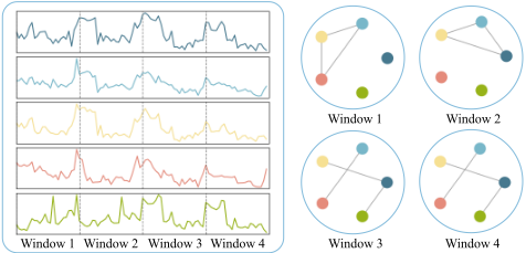
Dynamic nature of multivariate correlations: The relationships between variables are not static, and they can evolve over time, showing periodic or trend-based changes. As shown in Fig. 1, by treating time points as a time window, we observe that the correlation similarities vary across time windows. By learning from real sequence data, we can capture the dynamic relationships that evolve across different windows. Existing method (e.g., MTGNN [Wu et al., 2020]) has used a single graph to propagate correlation information across the entire time scale, and it fails to capture the varying correlation weights across different time windows. This limits the accuracy of feature aggregation based on overall sequence correlation, thereby affecting prediction precision.
Noise caused by negative relationships: Although existing methods (e.g., MSGNet [Cai et al., 2024]) have explored learnable graph structures, they often struggle to learn the optimal structure. This difficulty arises because realworld datasets are typically influenced by various unforeseen factors, which can cause uncorrelated variables to exhibit spurious similarities. As a result, these variables might propagate negative relationships (noise information) during the message-passing process, leading to model performance degradation. The noise can hinder the effective transmission of critical information between key variables, ultimately reducing the ability of model for capturing essential patterns.
To address the challenges outlined above, we propose a Dynamic Graph Learning Guided Multi-Scale Transformer (DGraFormer), which comprises two main components: Dynamic Correlation-aware Graph Learning (DCGL) and MultiScale Temporal Transformer (MTT). The method views time series data as multiple time windows with stable correlations. It adaptively learns the graph adjacency matrices for each time window, filters out noise, and selects the most crucial correlation weights to guide the aggregation of feature representations based on correlations. This approach significantly improves the ability of the model to adapt to dynamic correlation changes and overcomes the issue of redundant information propagation caused by external noise in existing methods. Our contributions are summarized in three main aspects:
- We propose a novel multivariate time series forecasting model, named DGraFormer, which combines DCGL and MTT in a unified framework to simultaneously achieve the dynamic correlation-aware graph learning and multi-scale temporal information interaction.
- A DCGL is designed to adaptively capture the dynamic correlations among multivariate variables in temporal windows, and then select essential information to guide the process of correlation feature aggregation, effectively eliminating noise in the weights and learning critical corresponding adjacency weights for dynamic graph learning.
- Extensive experiments on ten real-world datasets demonstrate that DGraFormer outperforms SOTA multivariate time series forecasting models. Compared to the latest graph-based model, MSGNet, our model achieves average reductions of 11% in MSE and 10.6% in MAE.
2 RelatedWork
2.1 Time Series Forecasting
Time series forecasting has been extensively studied. Recently, Transformer [Vaswani, 2017; Kitaev et al., 2020; Tang and Matteson, 2021] shows superior performance in semantic extraction and long-range dependency modeling, outperforming methods based on TCNs [Bai et al., 2018; Liu et al., 2022a; Lai et al., 2023] and RNNs [Rangapuram et al., 2018; Qin et al., 2017]. This trend drives interest in Transformer-based models. Informer [Zhou et al., 2021] has led the adoption of Transformer for time series forecasting. Autoformer [Wu et al., 2021] introduces seasonal trend decomposition, while FEDformer [Zhou et al., 2022] extends this approach by transforming the time domain into the frequency domain for decomposition learning. Pyraformer [Liu et al., 2022b] employs convolution to capture multi-scale features, and Non-stationary Transformers [Liu et al., 2022e] focus on time series stationarization.
Despite challenges raised by linear models [Zeng et al., 2023; Das et al., 2023], Transformers remain top-performing in time series forecasting [Jiang et al., 2023]. PatchTST [Nie et al., 2023] leverages channel independence by representing each variable as a separate channel and segmenting it into subsequence-level patches, which are subsequently used as tokens for the Transformer model. In contrast, Crossformer [Zhang and Yan, 2023] adopts variable patching and a hierarchical encoder-decoder to capture cross-dimensional dependencies. Recent work [Zhou et al., 2024a] proposes inputting the same number of auxiliary variables for each variable into the Transformer for learning. And iTransformer [Liu et al., 2024] encodes variables independently as distinct tokens, using attention for inter-variable and feedforward networks for temporal dependencies. Further techniques are under exploration [Pan et al., 2021; Deng et al., 2022; Li et al., 2023; Liu et al., 2023; Deng et al., 2024a; Deng et al., 2024b], including TimesNet [Wu et al., 2023], which projects one-dimensional time series data into a twodimensional space and analyzes it with sophisticated visual networks.
Most existing methods overlook the modeling of correlations between variables. Existing methods for learning variable correlations fail to account for the dynamic nature of multivariate correlations and the noise in correlation modeling. These approaches propagate information across all variables, while neglecting isolated variables (those not correlated with others).
2.2 GraphModeling for Multivariate Time Series Forecasting
The use of GNNs [Kipf and Welling, 2016; Defferrard et al., 2016; Abu-El-Haija et al., 2019] introduces a new perspective to model multivariate time series data. However, most existing approaches apply them to specific domains, such as traffic [Yu et al., 2017; Li et al., 2017; Wu et al., 2019; Wen et al., 2023; Liu et al., 2022c], where prior knowledge (e.g., Euclidean distance or POI) can naturally define graph structures. In contrast, general multivariate time series forecasting models involve datasets from multiple domains, making it difficult to obtain a unified, predefined graph structure.
To address this, some methods [Wu et al., 2020] have explored learnable graph structures, replacing predefined graphs with learnable parameter matrices. However, methods such as MAGNN [Chen et al., 2023] and MSGNet [Cai et al., 2024] still employ static graphs to represent time series, which are insufficient to capture the dynamic nature of variable correlations. Although TPGNN [Liu et al., 2022d] captures temporal dynamics through matrix polynomials, it ignores noise caused by external factors. Consequently, effectively learning the core correlations between variables remains a critical challenge in correlation modeling.
3 ProblemDefinition
For multivariate time series forecasting, we denote the input data over a look-back window as X = {x1, . . . , xT } ∈ RN×T , where T is the number of time steps and N is the number of variables. The objective is to forecast the next τ time steps, represented as Y = {xT+1, . . . , xT+τ } ∈ RN×τ .
We model the multivariate time series data using graphs G = {V, E}, where V denotes the set of nodes and E ∈ RN×N is the correlation weight matrix between the nodes. To capture the dynamic correlations between variables, we divide the time series data into W windows, each containing m time steps. The correlation graph structure is then represented as G = {V, {E1, E2, . . . , EW}}, where Ew ∈ RN×N is the correlation weight matrix for the w-th time window.
4 Methodology
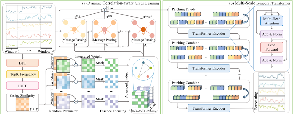
To effectively capture multivariate correlations, we propose a novel multivariate time series forecasting model called DGraFormer. The overall architecture of DGraFormer is illustrated in Fig. 2, comprising two main components: Dynamic correlation-aware graph Learning (DCGL) and MultiScale Temporal Transformer (MTT).
First, the DCGL generates the corresponding graph structure matrices with dynamic essential multivariate correlations for the input sequence. Then it takes the instance-normalized data and its corresponding edge weight matrices to learn the correlation representations. The MTT extracts temporal representations from the patch data at varying scales. Finally, the learned representations, which encapsulate both correlation and temporal information, are passed through the Flatten and Linear layers in the predictor to produce the final forecast output.
4.1 Dynamic Correlation-aware Graph Learning
The Dynamic Correlation-aware Graph Learning is designed to capture graph structures that reflect dynamic correlations and focus on essential correlation weights. We construct the weight matrix A ∈ RN×N×T , which guides the propagation of the correlation information for the input data X.
Dynamic Multivariate Correlation Weight Learning
Existing methods have modeled the entire time series with a single graph, which failed to capture dynamic changes in multivariate correlations. To overcome this limitation, and enable more precise correlation modeling, we divide the time series into W time windows, each containing m data points. For each time window, we independently learn its correlation graph weights.
First, we compute the overall correlation weights based on the information from the entire dataset used for training. It represents the general relationships between variables in the training set Xall ∈ RN×M , where M denotes the total number of time steps in the training set. Raw data is often influenced by trends and external factors, which complicates the extraction of the underlying correlations among variables masked by the overall trend. To mitigate these influences, we transform the data from the time domain to the frequency domain, removing trend components and extracting seasonal information. Specifically, we decompose Xall into Fourier bases using the Discrete Fourier Transform (DFT(·)), select the top Kf amplitudes, and apply the Inverse Discrete Fourier Transform (IDFT(·)) to obtain the seasonal representation of the data, denoted as Xsea ∈ RN×M :
where A is the set of amplitudes for all selected frequency components, and Φ is the set of phase angles for all selected frequency components. Using Xsea, we calculate the cosine similarity between all pairs of variables, which results in the overall matrix of correlation weights C ∈ RN×N :
Secondly, we generate a unique parametric correlation matrix for each time window and optimize it during the learning process. This enables precise modeling of variable correlations by capturing the fine-grained correlation graph structures within different time windows. Specifically, for the matrix of weights Rw ∈ RN×N of the w-th time window, it is computed as follows:
where (Ew)1 and (Ew)2 ∈ RN×h denote randomly initialized node embeddings (with each row corresponding to a variable). The subscripts 1 and 2 indicate different initialization instances, both of which are learnable during training. h is the embedding dimensionality.
Finally, we aggregate C and Rw to derive the correlation graph weights matrix Ew ∈ RN×N for the w-th time window:
where α governs the relative contribution of C to Ew. Initially, α is set to 0.9 and is gradually decreased to 0.1 as training progresses. This adjustment ensures that the parameterized weights matrix Rw progressively takes precedence over C in Ew, gradually reflecting the unique correlations among variables in the w-th time window.
Essential Correlation Information Focusing
To eliminate redundant information that may interfere with the learning of correlation features, such as temporary false correlations induced by external factors, and to focus on the essential correlation weights, we focus essential correlation information to Ew for each time window. Specifically, we generate a corresponding mask matrix Mw ∈ RN×N for the w-th time window by selecting the top Ke values from the vectorized form of Ew:
Given the learnable nature of Ew, Mw evolves dynamically during training, adaptively guiding the model in selecting the essential correlation weights. We apply the mask matrix to Ew as follows Ew :
where ˜ Ew ∈ RN×N denotes the sparsified correlation weight matrix for the w-th time window, and ⊙ indicates elementwise multiplication. We apply the above operation to the correlation edge weight matrix of each time window, obtaining a set of dynamically sparsified correlation edge weight matrices ˜ E = {˜ E1, ˜ E2, . . . , ˜ EW } ∈ RN×N×W .
For each input data X ∈ RN×T , we apply advanced indexing to extract the weight matrix A ∈ RN×N×T for correlation feature learning:
where I ∈ RT×1 denotes the index information of the time window for each time point. We then feed A into the GCNbased correlation fusion module to guide the information propagation process.
Correlation-aware Graph Message Passing
To propagate information based on the output weight matrix A, we use input data processed with Instance Norm, which is a technique used to mitigate distribution shifts between training and testing data, to learn feature representations that aggregate essential correlations. Inspired by MTGNN [Wu et al., 2020], we adopt a graph convolution approach that incorporates residual connections and the mix-hop concept for learning correlation representations. The information propagation step is defined as follows:
where H(0) denotes the input data X processed with Instance Normalization and feature dimensional upsampling, and H(l) represents the result of the l-th layer of message passing. β controls the proportion of the root node's original state retained, ensuring that the propagated node states explore the depth of the neighborhood while preserving locality. We use the following approach for information selection:
where the learnable parameter matrix W acts as a feature selector, and LMP represents the total number of layers for message passing. It adaptively selects the message passing features at different depths to generate the output Hout ∈ RN×T of the correlation fusion module.
4.2 Multi-Scale Temporal Transformer
The Multi-Scale Temporal Transformer is designed to capture the temporal patterns within sequence data. Existing methods, such as PatchTST [Nie et al., 2023], have shown that dividing time series into patches and using them as tokens in a Transformer Encoder for feature learning can significantly improve the accuracy of multivariate time series prediction. Aggregating time steps into subsequence-level patches enhances locality and captures comprehensive semantic information that cannot be obtained at the point level. However, using a single patch size to divide the time series overlooks the features present at different time resolutions. To address this, we adopt a multi-scale patch division and combination strategy to model temporal correlations.
Patch Division
For the output Hout ∈ RN×T of the correlation fusion module, we divide the i-th univariate time series hiout ∈ R1×T into S = T/P non-overlapping patches, where P represents the number of time steps in each patch, denoted as hip ∈ RP×S . We then apply a trainable linear projectionWp ∈ RD×P to map the patches to the Transformer latent space of dimension D. In addition, we use a learnable additive position encoding Wpos ∈ RD×S to capture the temporal order of the patches:
where ¯xi ∈ RD×S denotes the univariate input to the Transformer encoder.
Transformer Encoder
The structure of our transformer encoder follows the standard vanilla Transformer architecture. Initially, the multihead self-attention mechanism is used to model the temporal correlations between different patches. By applying a linear transformation to the input ¯xi , we obtain the query, key, and value matrices, denoted as Qi ,Ki ,Vi . The attention output zia ∈ RD×S is then computed as follows:
Subsequently, the attention output is processed through the Add & Norm layer, which integrates residual connections and batch normalization to improve training stability and convergence. This operation can be mathematically expressed as:
where Norm(·) denotes the BatchNorm. Following the Add & Norm layer, the intermediate representation is further refined using a position-wise feed-forward network (FFN). The FFN is composed of two linear transformations separated by a non-linear activation function. The output of this stage is given by:
As a result, the transformer encoder produces the multivariate output Z ∈ RN×D×S , which encapsulates the temporal feature representation of the input sequence.
Patch Combination and Multi-Scale Encoding
To capture the diverse features embedded in multi-scale patches, we combine neighboring patches pairwise and input them into another identical Transformer encoder for further learning. This process is represented as:
where Z(l) ∈ RN×D(l)×S(l) represents the output of the lth layer of the transformer encoder TE(l) (·), which includes multi-head attention, BatchNorm layers, and feed-forward network. The input to the first encoder TE0 (·) is denoted as X(0) p , and its output as Z(0) . Through multiple iterations, we learn feature representations that capture information across different time resolutions. Finally, After being processed by LTE layers of Transformer encoder, the output of the last Transformer encoder is flattened, and a Linear layer is applied to generate the final prediction result Y = {xT+1, . . . , xT+τ } ∈ RN×τ .
5 Experiments
The experiments are designed to address the following research questions:
- RQ1: What is the performance of our DGraFormer as compared to various state-of-the-art baselines?
- RQ2: How do the key components contribute to the performance?
- RQ3: How do the key hyperparameters influence the performance of the proposed DGraFormer?
5.1 Datasets
In our experimental evaluation, we employ 10 real-world datasets, including ETT (4 subsets), Weather, Electricity, Solar-Energy, Traffic used by iTransformer [Liu et al., 2024], Flight evaluated in MSGNet [Cai et al., 2024] and AirQualityUCI 1 , to assess the performance of all methods.
5.2 Baselines
We compare our DGraFormer against with four categories of baselines: (1) Graph-based method: MSGNet [Cai et al., 2024]; (2) Transformer-based methods: iTransformer [Liu et al., 2024], PatchTST [Nie et al., 2023], Crossformer [Zhang and Yan, 2023], Pyraformer [Liu et al., 2022b]; (3) Linearbased methods: DLinear [Zeng et al., 2023], TiDE [Das et al., 2023]; (4) TCN-based method: TimesNet [Wu et al., 2023].
5.3 Experiment Settings and EvaluationMetrics
DGraFormer uses the Adam optimizer and a combination of L1 and L2 loss for model training. The number LMP of graph message passing layers is set to 2, and the number LTE of the Transformer encoder is set to 3. Additionally, a patch length p = 8 is used for division. The number of time points m in each time window depends on the dataset's time frequency, corresponding to the number of data points in one day (e.g., 24 for Electricity, 144 for Solar). The weight focusing ratio Ke ranges from 0.5 to 0.005 based on the number of variables in the dataset, decreasing as the number of variables increases. And we set Kf=3 in Eq. (1). All experiments are conducted using PyTorch and executed on an NVIDIA GeForce RTX 4090 24GB GPU. To ensure fair comparisons, all models are configured with the same look-back window T = 96 and prediction lengths τ ∈ {96, 192, 336, 720} for all datasets. The hyperparameters for the baseline models are set according to the configurations provided in the original papers. We evaluate model performance using two common metrics in multivariate time series forecasting: Mean Absolute Error (MAE) and Mean Squared Error (MSE).
1 https://github.com/Gauhar1107/AirQualityUCI
| Models | Ours | iTransformer (ICLR2024) | MSGNet (AAAI2024) | PatchTST (ICLR2023) | TimesNet (ICLR2023) | TIDE (arXiv2023) | Dlinear (AAAI2023) | Crossformer (ICLR2023) | Pyraformer (ICLR2022) | ||||||||||||||||
|---|---|---|---|---|---|---|---|---|---|---|---|---|---|---|---|---|---|---|---|---|---|---|---|---|---|
| Metric | MSE | MAE | MSE | MAE | MSE | MAE | MSE | MAE | MSE | MAE | MSE | MAE | MSE | MAE | MSE | MAE | MSE | MAE | |||||||
| 96 | 0.367 | 0.393 | 0.386 | 0.405 | 0.390 | 0.411 | 0.414 | 0.419 | 0.384 | 0.402 | 0.479 | 0.464 | 0.386 | 0.400 | 0.423 | 0.448 | 0.664 | 0.612 | |||||||
| 192 | 0.438 | 0.426 | 0.441 | 0.436 | 0.442 | 0.442 | 0.460 | 0.445 | 0.436 | 0.429 | 0.525 | 0.492 | 0.437 | 0.432 | 0.471 | 0.474 | 0.790 | 0.681 | |||||||
| 336 ETTh1 | 0.479 | 0.442 | 0.487 | 0.458 | 0.480 | 0.468 | 0.501 | 0.466 | 0.491 | 0.469 | 0.565 | 0.515 | 0.481 | 0.459 | 0.570 | 0.546 | 0.891 | 0.738 | |||||||
| 720 | 0.484 | 0.467 | 0.503 | 0.491 | 0.494 | 0.488 | 0.500 | 0.488 | 0.521 | 0.500 | 0.594 | 0.558 | 0.519 | 0.516 | 0.653 | 0.622 | 0.963 | 0.782 | |||||||
| 96 | 0.300 | 0.344 | 0.297 | 0.349 | 0.328 | 0.371 | 0.302 | 0.348 | 0.340 | 0.374 | 0.400 | 0.440 | 0.333 | 0.387 | 0.584 | 0.645 | 0.597 | ||||||||
| 192 | 0.382 | 0.397 | 0.380 | 0.400 | 0.402 | 0.414 | 0.388 | 0.400 | 0.402 | 0.414 | 0.528 | 0.509 | 0.477 | 0.476 | 0.745 0.877 | 0.656 | 0.788 | 0.683 | |||||||
| 336 ETTh2 | 0.388 | 0.415 | 0.428 | 0.432 | 0.435 | 0.443 | 0.426 | 0.433 | 0.452 | 0.452 | 0.643 | 0.517 | 0.594 | 0.541 | 1.043 | 0.7731 | 0.907 | 0.747 | |||||||
| 720 | 0.418 | 0.436 | 0.427 | 0.445 | 0.417 | 0.441 | 0.431 | 0.446 | 0.462 | 0.468 | 0.874 | 0.679 | 0.831 | 0.657 | 1.104 | 0.763 | 0.963 | 0.783 | |||||||
| 96 | 0.326 | 0.366 | 0.334 | 0.368 | 0.319 | 0.366 | 0.329 | 0.367 | 0.338 | 0.375 | 0.364 | 0.387 | 0.345 | 0.372 | 0.404 | 0.426 | 0.543 | 0.510 | |||||||
| 0.450 | 0.557 | ||||||||||||||||||||||||
| 192 | 0.358 | 0.376 | 0.377 | 0.391 | 0.376 | 0.397 | 0.367 | 0.385 | 0.374 | 0.387 | 0.398 | 0.404 | 0.380 | 0.389 | 0.451 | 0.537 | |||||||||
| 336 ETTm1 | 0.387 | 0.397 | 0.426 | 0.420 | 0.417 | 0.422 | 0.399 | 0.410 | 0.410 | 0.411 | 0.428 | 0.413 | 0.413 | 0.515 | 0.754 | 0.655 | |||||||||
| 720 | 0.446 | 0.436 | 0.491 | 0.459 | 0.481 | 0.458 | 0.454 | 0.439 | 0.478 | 0.450 | 0.487 | 0.425 0.461 | 0.474 | 0.453 | 0.532 0.666 | 0.589 | 0.908 | 0.724 | |||||||
| 96 | 0.173 | 0.253 | 0.180 | 0.264 | 0.177 | 0.262 | 0.175 | 0.259 | 0.187 | 0.267 | 0.207 | 0.305 | 0.193 | 0.292 | 0.287 | 0.366 | 0.435 | 0.507 | |||||||
| 192 | 0.243 | 0.302 | 0.250 | 0.309 | 0.247 | 0.307 | 0.241 | 0.302 | 0.249 | 0.309 | 0.290 | 0.364 | 0.284 | 0.362 | 0.492 | 0.730 | 0.673 | ||||||||
| 336 ETTm2 | 0.315 | 0.348 | 0.311 | 0.348 | 0.312 | 0.346 | 0.305 | 0.343 | 0.321 | 0.351 | 0.377 | 0.422 | 0.369 | 0.427 | 0.414 0.597 | 0.542 | 1.201 | 0.845 | |||||||
| 720 | 0.404 | 0.401 | 0.412 | 0.407 | 0.414 | 0.403 | 0.402 | 0.400 | 0.408 | 0.403 | 0.558 | 0.524 | 0.554 | 0.522 | 1.730 | 1.042 | 3.625 | 1.451 | |||||||
| 96 | 0.168 | 0.207 | 0.174 | 0.214 | 0.163 | 0.212 | 0.177 | 0.218 | 0.172 | 0.220 | 0.202 | 0.261 | 0.196 | 0.255 | 0.230 | 0.896 | 0.556 | ||||||||
| 192 | 0.213 | 0.249 | 0.221 | 0.254 | 0.212 | 0.254 | 0.225 | 0.259 | 0.219 | 0.261 | 0.242 | 0.298 | 0.296 | 0.158 0.206 | 0.277 | 0.622 | 0.624 | ||||||||
| 336 Weather | 0.270 | 0.291 | 0.278 | 0.296 | 0.272 | 0.299 | 0.278 | 0.297 | 0.280 | 0.306 | 0.287 | 0.237 | 0.335 | 0.272 | 0.335 | 0.739 | 0.753 | ||||||||
| 0.358 | 0.349 | 0.335 | 0.283 | 0.398 | |||||||||||||||||||||
| 720 | 0.345 | 0.338 | 0.350 | 0.348 | 0.354 | 0.348 | 0.365 | 0.359 | 0.351 | 0.386 | 0.345 | 0.381 | 0.418 | 1.004 | 0.934 | ||||||||||
| 96 | 0.136 | 0.229 | 0.148 | 0.240 | 0.165 | 0.274 | 0.195 | 0.285 | 0.168 | 0.272 | 0.237 | 0.329 | 0.197 | 0.282 | 0.219 | 0.314 | 0.386 0.386 | 0.449 | |||||||
| 192 Electricity | 0.155 | 0.244 | 0.162 | 0.253 | 0.184 | 0.292 | 0.199 | 0.289 | 0.184 | 0.289 | 0.236 | 0.330 | 0.196 | 0.285 | 0.231 | 0.322 | 0.443 | ||||||||
| 336 | 0.171 | 0.261 | 0.178 | 0.269 | 0.195 | 0.302 | 0.215 | 0.305 | 0.198 | 0.300 | 0.249 | 0.344 | 0.209 | 0.301 | 0.246 | 0.337 | 0.378 | 0.443 | |||||||
| 720 96 | 0.210 0.184 | 0.298 0.219 | 0.225 0.203 | 0.317 0.237 | 0.231 0.259 | 0.332 | 0.256 0.234 | 0.337 0.286 | 0.220 0.250 | 0.320 0.292 | 0.284 | 0.373 0.399 | 0.245 0.290 | 0.333 0.378 | 0.280 0.310 | 0.363 0.331 | 0.218 | 0.445 0.274 | |||||||
| 0.285 | 0.310 | 0.296 | 0.312 | 0.416 | 0.320 | 0.734 | 0.725 | ||||||||||||||||||
| 192 Solar | 0.211 | 0.234 | 0.233 | 0.261 | 0.268 | 0.293 | 0.267 | 0.318 | 0.339 | 0.398 | 0.750 | 0.227 | 0.284 | ||||||||||||
| 336 | 0.234 | 0.250 | 0.248 | 0.273 | 0.316 | 0.326 | 0.290 | 0.315 | 0.319 | 0.330 | 0.368 | 0.430 | 0.353 | 0.415 | 0.735 | 0.246 | 0.296 | ||||||||
| 720 96 | 0.235 0.442 | 0.254 0.245 | 0.249 0.395 | 0.275 0.268 | 0.313 0.598 | 0.326 | 0.289 | 0.317 | 0.388 | 0.337 0.321 | 0.370 0.805 | 0.425 0.493 | 0.356 0.650 | 0.413 0.396 | 0.769 0.522 | 0.765 0.290 | 0.252 2.085 | 0.296 0.468 | |||||||
| 192 | 0.417 | 0.339 | 0.544 0.540 | 0.359 0.354 | 0.593 | 0.530 | |||||||||||||||||||
| Traffic | 0.469 | 0.257 | 0.276 | 0.616 | 0.358 | 0.617 | 0.336 | 0.756 | 0.474 | 0.598 | 0.370 | 0.293 | 0.867 | 0.467 | |||||||||||
| 336 | 0.433 | 0.358 | 0.477 | 0.605 | 0.469 | ||||||||||||||||||||
| 0.481 | 0.266 | 0.283 | 0.651 | 0.373 | 0.511 | 0.629 | 0.336 | 0.762 | 0.373 | 0.305 | 0.869 | ||||||||||||||
| 720 96 | 0.510 0.143 | 0.281 0.250 | 0.467 0.144 | 0.302 | 0.699 | 0.404 | 0.586 0.175 | 0.375 0.305 | 0.640 0.237 | 0.350 0.350 | 0.719 0.225 | 0.449 | 0.645 | 0.394 | 0.558 0.589 0.151 | 0.328 | 0.229 | 0.473 0.343 | 0.337 | ||||||
| 192 | 0.143 | 0.247 | 0.147 | 0.252 0.253 | 0.183 0.189 | 0.301 | 0.176 | 0.304 | 0.224 | 0.337 | 0.225 | 0.341 0.340 | 0.221 0.220 | 0.336 | 0.159 | 0.259 0.264 | 0.248 | 0.357 | |||||||
| Flight | 0.159 | 0.266 | 0.306 | 0.187 | 0.314 | 0.289 | 0.394 | 0.235 | 0.342 | 0.285 | 0.413 | ||||||||||||||
| 336 | 0.154 | 0.291 | 0.297 | 0.253 | 0.358 | 0.228 | 0.272 | 0.263 | 0.366 | 0.329 | 0.606 | ||||||||||||||
| 720 | 0.191 | 0.257 | 0.193 | 0.206 | 0.320 | 0.343 | 0.310 | 0.408 | 0.347 0.373 | 0.229 | 0.178 0.203 | 0.307 | 0.656 1.350 | 0.750 | |||||||||||
| 96 | 1.147 | 1.192 | 0.601 | 1.232 | 0.616 | 1.240 | 0.620 | 1.203 | 0.607 | 1.309 | 1.303 | 0.682 | 1.177 | 0.621 | |||||||||||
| 192 | 1.238 | 0.580 0.606 | 1.308 | 1.350 | 0.658 | 1.337 | 0.644 | 1.330 | 1.472 | 0.650 0.688 | 1.385 | 0.702 | 1.321 | 0.665 | 1.607 | 0.824 | |||||||||
| AirQualityUCI | 0.633 | 0.675 | 1.408 | 0.660 | 1.466 | 0.645 | 1.445 | 0.709 | 1.468 | 0.722 | 0.707 | 1.600 1.807 | 0.795 | ||||||||||||
| 336 720 | 1.344 1.482 | 0.644 0.696 | 1.401 1.532 | 0.659 0.708 | 1.490 1.592 | 0.717 | 1.609 | 0.726 | 1.580 | 0.673 0.704 | 1.572 1.806 | 0.777 | 1.721 | 0.813 | 1.599 | 0.763 | 0.889 | ||||||||
5.4 Experiment Results
Performance Comparison (RQ1)
The results of multivariate time series forecasting are presented in Table 1, DGraFormer achieves optimal performance on most of the evaluation metrics. Compared with 2024 SOTA models iTransformer and MSGNet, DGraFormer reduces MSE and MAE by an average of 6.75% and 7.25%. All models face performance decline with longer prediction lengths due to information decay and error accumulation. Yet DGraFormer consistently outperforms SOTA, e.g., exceeding MSGNet by 10.5%/10.8% (MSE/MAE) at horizon=192, 11.7%/11.0% at 336, and 10.5%/9.8% at 720. This demonstrates its robust capability in long-term forecasting.
Specifically, on high-dimensional datasets (Electricity, Solar, Traffic) with 100+ variables, DGraFormer reduces MAE by 6.6% over iTransformer by (1) capturing richer intervariable correlations via graph attention and (2) leveraging more contextual information for improved accuracy. Although Transformer-based models (e.g., iTransformer) employ multi-head attention to capture inter-variable correlations, they do not explicitly model multivariate correlations. In contrast, graph-based methods more flexibly model dynamic, complex variable correlations. iTransformer uses shared attention across variables, limiting its ability to capture evolving, heterogeneous correlations in multivariate series.
Despite both using graph-based correlation modeling, DGraFormer outperforms MSGNet by 11% MSE and 10.6% MAE on average. On MSGNet's FLight dataset, DGraFormer reduces MSE by 24% and MAE by 18.7%. While MSGNet learns graph structures across multiple scales, it does not dynamically model within each scale or handle noise effectively. This demonstrates that dynamic modeling and focusing on key correlations can significantly improve forecast accuracy.
Compared with linear-based models TiDE and DLinear, DGraFormer reduces MSE/MAE by 21.7%/17.9%. This further confirms that a well-designed Transformer model can still achieve strong performance in time series forecasting.
Ablation Study (RQ2)
We ablate DGraFormer's components with four variants:
- w/o Dynamic Time Windows (DTW): Using a single graph to learn variable correlations across all time steps.
- w/o Dynamic Graph Learning (DGL): Using only the initial adjacency matrix C to model variable correlations.
- w/o Essential Correlation Weight Focusing (ECF): Using all positive weights for graph message propagation.
- w/o Multi-scale Transformer Encoding (MTE): Using a fixed uniform patch size across all Transformer encoder layers for temporal learning, without patch combination.
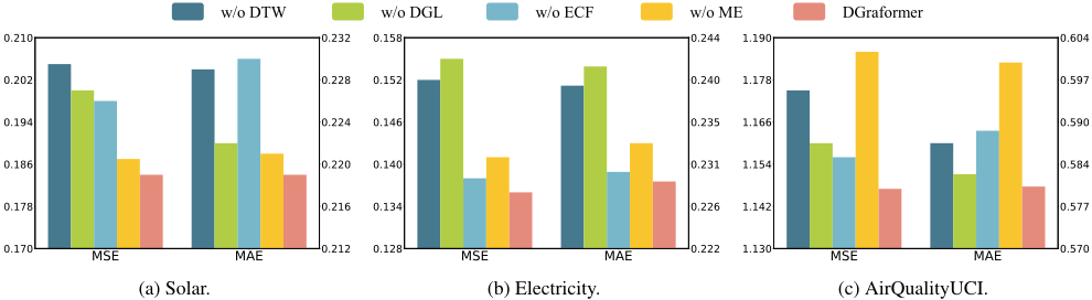
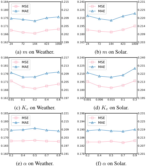
Fig. 3 illustrates the predictive performance of different model variants on Solar, Electricity, and AirQualityUCI datasets. Removing the dynamic time window caused a substantial decrease in accuracy, highlighting the importance of modeling dynamic correlations in inter-variable relationships. The removal of dynamic graph learning impairs the model's ability to adaptively capture correlations among variables. Excluding the essential correlation weight focusing resulted in the model's inability to effectively filter out noise, which disrupted the communication of core correlations. Finally, removing multi-scale encoding restricted the model's capacity to capture time features at different scales. Overall, graph learning effectively captures the correlations between variables, while the Transformer excels in learning temporal features across different time scales. The combination of these components results in improved prediction performance.
Parameter Sensitivity Analysis (RQ3)
We analyze the parameter sensitivity of DGraFormer with respect to three key hyperparameters, the number m of time points, the weight focusing ratio Ke, and the cosine similarity matrix proportion α on Weather and Solar datasets.
Fig. 4a and 4b show the prediction performance for varying values of m, the number of time points in each time window. The model performs best when m = 144, corresponding to a full day, as correlations within a single day may tend to be stable. Larger time windows, however, introduce varying correlations, reducing performance.
Fig. 4c and 4d assess the impact of the weight focusing ratio Ke. As Ke decreases, performance improves up to a point before declining. A moderate decrease helps eliminate redundant noise, preserving essential correlations for accurate feature aggregation. However, too low a Ke discards important weights, weakening model performance.
Fig. 4e and 4f assess the cosine similarity matrix proportion α. Performance remains stable across α values, as graph structure learning adaptively adjusts weights to mitigate fluctuations. The cosine similarity matrix helps prevent random initialization fitting issues and guides the model to adjust based on a correlation matrix that reflects seasonal patterns. Graph learning compensates for changes introduced by varying retention ratios.
6 Conclusion
In this paper, we propose the Dynamic Graph Learning Guided Multi-Scale Transformer (DGraFormer) to address challenges in multivariate time series forecasting. The model integrates two key components: Dynamic Correlation-aware Graph Learning (DCGL), which captures dynamic correlations and filters noise, and Multi-Scale Temporal Feature Learning (MTF), which extracts temporal patterns at multiple scales. Experimental results demonstrate that DGraFormer outperforms sota methods on ten real-world datasets, achieving superior performance.
Acknowledgments
This work is partially supported by the National Natural Science Foundation of China under Grant Nos. 62176243, 62372421, and 62402463, the Fundamental Research Funds for the Central Universities under Grant No. 202442005, and the National Key R&D Program of China under Grant No. 2022ZD0117201.
@inproceedings{ijcai2025p391,
  title     = {DGraFormer: Dynamic Graph Learning Guided Multi-Scale Transformer for Multivariate Time Series Forecasting},
  author    = {Yan, Han and Chen, Dongliang and Jiang, Guiyuan and Wang, Bin and Cao, Lei and Dong, Junyu and Yu, Yanwei},
  booktitle = {Proceedings of the Thirty-Fourth International Joint Conference on
               Artificial Intelligence, {IJCAI-25}},
  publisher = {International Joint Conferences on Artificial Intelligence Organization},
  editor    = {James Kwok},
  pages     = {3516--3524},
  year      = {2025},
  month     = {8},
  note      = {Main Track},
  doi       = {10.24963/ijcai.2025/391},
  url       = {https://doi.org/10.24963/ijcai.2025/391},
}
TY - CPAPER TI - DGraFormer: Dynamic Graph Learning Guided Multi-Scale Transformer for Multivariate Time Series Forecasting AU - Yan, Han AU - Chen, Dongliang AU - Jiang, Guiyuan AU - Wang, Bin AU - Cao, Lei AU - Dong, Junyu AU - Yu, Yanwei T2 - Proceedings of the Thirty-Fourth International Joint Conference on Artificial Intelligence, IJCAI-25 PB - International Joint Conferences on Artificial Intelligence Organization PY - 2025 SP - 3516 EP - 3524 DO - 10.24963/ijcai.2025/391 UR - https://doi.org/10.24963/ijcai.2025/391 ER -Copied
Machine-readable versions of this paper, for tools and AI agents:





