
Addressing Downward Memory Loss in Hierarchical GNN Forecasters Through Memory-Buffered Decoding
Proceedings of the Thirty-Fifth International Joint Conference on Artificial Intelligence. Main Track. Pages 4152-4160.
https://doi.org/10.24963/ijcai.2026/462
Keywords
- Machine Learning: Time series and data streams
- Machine Learning: Sequence and graph learning
- Machine Learning: Multi-view learning
- Machine Learning: Learning graphical models
Abstract
Accurate spatio-temporal forecasting requires modeling interactions across multiple spatial and temporal scales. Existing Graph Neural Network (GNN) forecasters primarily operate at a single local scale, limiting their ability to capture global processes that govern system dynamics. Hierarchical GNNs (HGNNs) aim to address this limitation by learning multiscale representations, but in practice, they often fail to preserve global information during coarse-to-fine propagation. We identify this limitation as downward memory loss, where global trends learned at coarse resolutions diminish before influencing fine-grained predictions, leading to misaligned local dynamics. We propose HiGFlow, an HGNN forecaster that explicitly preserves multiscale trends through a self-updating memory buffer that integrates into the coarse-to-fine information flow. This design maintains global contextual signals as an inductive bias throughout hierarchical decoding. We provide a theoretical analysis indicating that when decoding, HiGFlow preserves multiscale trends where residual-based architectures may fail to do so. Empirically, HiGFlow achieves substantially lower MAE and RMSE than state-of-the-art forecasting models across multiple benchmark datasets, demonstrating the importance of explicit global memory in multiscale spatio-temporal forecasting. Our implementation is available at https://github.com/TB862/HiGFlow.
- [Bauer et al., 2015] Peter Bauer, Alan Thorpe, and Gilbert Brunet. The quiet revolution of numerical weather pre- diction. Nature, 525(7567):47-55, 2015.
- [Cai et al., 2024] Wanlin Cai, Kun Wang, Hao Wu, Xiaoxu Chen, and Yuankai Wu. Forecastgrapher: Redefining multivariate time series forecasting with graph neural net- works. Advances in Neural Information Processing Sys- tems, 2024.
- [Cao et al., 2020] Defu Cao, Yujing Wang, Juanyong Duan, Ce Zhang, Xia Zhu, Congrui Huang, Yunhai Tong, Bix- iong Xu, Jing Bai, Jie Tong, et al. Spectral temporal graph neural network for multivariate time-series forecast- ing. Advances in Neural Information Processing Systems, 33:17766-17778, 2020.
- [Chen et al., 2020] Deli Chen, Yankai Lin, Wei Li, Peng Li, Jie Zhou, and Xu Sun. Measuring and relieving the over- smoothing problem for graph neural networks from the topological view. In Proceedings of the AAAI conference on artificial intelligence, volume 34, pages 3438-3445, 2020.
- [Cini et al., 2023] Andrea Cini, Danilo Mandic, and Cesare Alippi. Graph-based time series clustering for end-to- end hierarchical forecasting. International Conference on Learning Representations, 2023.
- [Cui et al., 2025] Jiaxu Cui, Qipeng Wang, Yiming Zhao, Bingyi Sun, Pengfei Wang, and Bo Yang. State feedback enhanced graph differential equations for multivariate time series forecasting. In James Kwok, editor, Proceedings of the Thirty-Fourth International Joint Conference on Arti- ficial Intelligence (IJCAI-25), pages 7374-7382. Interna- tional Joint Conferences on Artificial Intelligence Organi- zation, August 2025. Main Track. IJCAI
- [Guo et al., 2021] Kan Guo, Yongli Hu, Yanfeng Sun, Sean Qian, Junbin Gao, and Baocai Yin. Hierarchical graph convolution network for traffic forecasting. In Proceed- ings of the AAAI conference on artificial intelligence, vol- ume 35, pages 151-159, 2021.
- [Hu et al., 2025] Yifan Hu, Peiyuan Liu, Peng Zhu, Dawei Cheng, and Tao Dai. Adaptive multi-scale decomposition framework for time series forecasting. In Proceedings of the AAAI Conference on Artificial Intelligence, volume 39, pages 17359-17367, 2025.
- [Jin et al., 2025] Ming Jin, Guangsi Shi, Yuan-Fang Li, Bo Xiong, Tian Zhou, Flora D. Salim, Liang Zhao, Lingfei Wu, Qingsong Wen, and Shirui Pan. Towards expressive spectral-temporal graph neural networks for time series forecasting. IEEE Transactions on Pattern Analysis and Machine Intelligence, 47:4926-4939, 2025.
- [Karimi et al., 2021] Ahmad Maroof Karimi, Yinghui Wu, Mehmet Koyuturk, and Roger H French. Spatiotemporal graph neural network for performance prediction of pho- tovoltaic power systems. In Proceedings of the AAAI con- ference on artificial intelligence, volume 35, pages 15323- 15330, 2021.
- [Lam et al., 2023] Remi Lam, Alvaro Sanchez-Gonzalez, Matthew Willson, Peter Wirnsberger, Meire Fortunato, Ferran Alet, Suman Ravuri, Timo Ewalds, Zach Eaton- Rosen, Weihua Hu, Alexander Merose, Stephan Hoyer, George Holland, Oriol Vinyals, Jacklynn Stott, Alexan- der Pritzel, Shakir Mohamed, and Peter Battaglia. Learn- ing skillful medium-range global weather forecasting. Sci- ence, 382(6677):1416-1421, 2023.
- [Lan et al., 2022] Shiyong Lan, Yitong Ma, Weikang Huang, Wenwu Wang, Hongyu Yang, and Pyang Li. Dstagnn: Dynamic spatial-temporal aware graph neural network for traffic flow forecasting. In International conference on ma- chine learning, pages 11906-11917. PMLR, 2022.
- [Liu et al., 2024] Yong Liu, Tengge Hu, Haoran Zhang, Haixu Wu, Shiyu Wang, Lintao Ma, and Mingsheng Long. itransformer: Inverted transformers are effective for time series forecasting. International Conference on Learning Representations, 2024.
- [Luo et al., 2025] Yicheng Luo, Bowen Zhang, Zhen Liu, and Qianli Ma. Hi-patch: Hierarchical patch GNN for irregular multivariate time series. In Aarti Singh, Maryam Fazel, Daniel Hsu, Simon Lacoste-Julien, Fe- lix Berkenkamp, Tegan Maharaj, Kiri Wagstaff, and Jerry Zhu, editors, Proceedings of the 42nd International Con- ference on Machine Learning, volume 267 of Proceed- ings of Machine Learning Research, pages 41494-41519. PMLR, 13-19 Jul 2025.
- [Nie et al., 2023] Yuqi Nie, Nam H Nguyen, Phanwadee Sinthong, and Jayant Kalagnanam. A time series is worth 64 words: Long-term forecasting with transformers. Inter- national Conference on Learning Representations, 2023.
- [Oskarsson et al., 2024] Joel Oskarsson, Tomas Landelius, Marc Peter Deisenroth, and Fredrik Lindsten. Probabilis- tic weather forecasting with hierarchical graph neural net- works. In The Thirty-eighth Annual Conference on Neural Information Processing Systems, 2024.
- [Rusch et al., 2023] T Konstantin Rusch, Michael M Bron- stein, and Siddhartha Mishra. A survey on over- smoothing in graph neural networks. arXiv preprint arXiv:2303.10993, 2023.
- [Wang et al., 2025a] Shiyu Wang, Jiawei Li, Xiaoming Shi, Zhou Ye, Baichuan Mo, Wenze Lin, Shengtong Ju, Zhix- uan Chu, and Ming Jin. Timemixer++: A general time series pattern machine for universal predictive analysis. International Conference on Learning Representations, 2025.
- [Wang et al., 2025b] Yulong Wang, Yushuo Liu, Xiaoyi Duan, and Kai Wang. Filterts: Comprehensive frequency filtering for multivariate time series forecasting. In Pro- ceedings of the AAAI Conference on Artificial Intelligence, volume 39, pages 21375-21383, 2025.
- [Wu et al., 2021] Haixu Wu, Jiehui Xu, Jianmin Wang, and Mingsheng Long. Autoformer: Decomposition transform- ers with auto-correlation for long-term series forecast- ing. Advances in neural information processing systems, 34:22419-22430, 2021.
- [Wu et al., 2022] Lingfei Wu, Peng Cui, Jian Pei, Liang Zhao, and Xiaojie Guo. Graph neural networks: founda- tion, frontiers and applications. In Proceedings of the 28th ACM SIGKDD Conference on Knowledge Discovery and Data Mining, pages 4840-4841, 2022.
- [Wu et al., 2023a] Haixu Wu, Tengge Hu, Yong Liu, Hang Zhou, Jianmin Wang, and Mingsheng Long. Timesnet: Temporal 2d-variation modeling for general time series analysis. International Conference on Learning Represen- tations, 2023.
- [Wu et al., 2023b] Qitian Wu, Chenxiao Yang, Wentao Zhao, Yixuan He, David Wipf, and Junchi Yan. Dif- former: Scalable (graph) transformers induced by energy constrained diffusion. arXiv preprint arXiv:2301.09474, 2023.
- [Wu et al., 2023c] Xinyi Wu, Amir Ajorlou, Zihui Wu, and Ali Jadbabaie. Demystifying oversmoothing in attention- based graph neural networks. Advances in Neural Infor- mation Processing Systems, 36:35084-35106, 2023.
- [Xu et al., 2019] Keyulu Xu, Weihua Hu, Jure Leskovec, and Stefanie Jegelka. How powerful are graph neural net- works? International Conference on Learning Represen- tations, 2019.
- [Yan et al., 2024] Jielong Yan, Yifan Feng, Shihui Ying, and Yue Gao. Hypergraph dynamic system. In International Conference on Learning Representations, 2024.
- [Yan et al., 2025] Han Yan, Dongliang Chen, Guiyuan Jiang, Bin Wang, Lei Cao, Junyu Dong, and Yanwei Yu. Dgraformer: Dynamic graph learning guided multi-scale transformer for multivariate time series forecasting. In James Kwok, editor, Proceedings of the Thirty-Fourth International Joint Conference on Artificial Intelligence (IJCAI-25), pages 3516-3524. International Joint Con- ferences on Artificial Intelligence Organization, August 2025. Main Track. IJCAI
- [Yang et al., 2021] Jinyu Yang, Peilin Zhao, Yu Rong, Chaochao Yan, Chunyuan Li, Hehuan Ma, and Junzhou Huang. Hierarchical graph capsule network. In Proceed- ings of the AAAI Conference on Artificial Intelligence, vol- ume 35, pages 10603-10611, 2021.
- [Ye et al., 2022] Junchen Ye, Zihan Liu, Bowen Du, Leilei Sun, Weimiao Li, Yanjie Fu, and Hui Xiong. Learning the evolutionary and multi-scale graph structure for mul- tivariate time series forecasting. In Proceedings of the 28th ACM SIGKDD conference on knowledge discovery and data mining, pages 2296-2306, 2022.
- [Yi et al., 2024a] Kun Yi, Qi Zhang, Wei Fan, Hui He, Liang Hu, Pengyang Wang, Ning An, Longbing Cao, and Zhen- dong Niu. Fouriergnn: Rethinking multivariate time series forecasting from a pure graph perspective. Advances in Neural Information Processing Systems, 36, 2024.
- [Yi et al., 2024b] Kun Yi, Qi Zhang, Wei Fan, Shoujin Wang, Pengyang Wang, Hui He, Ning An, Defu Lian, Longbing Cao, and Zhendong Niu. Frequency-domain mlps are more effective learners in time series forecast- ing. Advances in Neural Information Processing Systems, 36, 2024.
- [Zeng et al., 2023] Ailing Zeng, Muxi Chen, Lei Zhang, and Qiang Xu. Are transformers effective for time series fore- casting? In Proceedings of the AAAI conference on artifi- cial intelligence, volume 37, pages 11121-11128, 2023.
- [Zhang et al., 2021] Xiang Zhang, Marko Zeman, Theodoros Tsiligkaridis, and Marinka Zitnik. Graph- guided network for irregularly sampled multivariate time series. International Conference on Learning Representations, 2021.
- [Zhou et al., 2021] Haoyi Zhou, Shanghang Zhang, Jieqi Peng, Shuai Zhang, Jianxin Li, Hui Xiong, and Wan- cai Zhang. Informer: Beyond efficient transformer for long sequence time-series forecasting. In Proceedings of the AAAI conference on artificial intelligence, volume 35, pages 11106-11115, 2021.
- [Zhou et al., 2022] Tian Zhou, Ziqing Ma, Qingsong Wen, Xue Wang, Liang Sun, and Rong Jin. Fedformer: Fre- quency enhanced decomposed transformer for long-term series forecasting. In International conference on machine learning, pages 27268-27286. PMLR, 2022.
References were extracted automatically from the PDF and may contain errors.
Full text extracted automatically from the PDF; figures, tables and equations may differ. The PDF is the version of record.
1 Introduction
Spatio-temporal forecasting requires modeling interactions that evolve across multiple spatial and temporal scales. Graph Neural Networks (GNNs) have become a key tool for modeling local dependencies in domains such as weather prediction [Lam et al., 2023; Bauer et al., 2015], traffic flow [Lan et al., 2022], and power grid forecasting [Karimi et al., 2021]. However, single resolution models struggle to reconcile fine-grained variability with broader global processes, which jointly determine system evolution. Accurate forecasting requires maintaining alignment between local patterns and the global drivers that influence their dynamics.
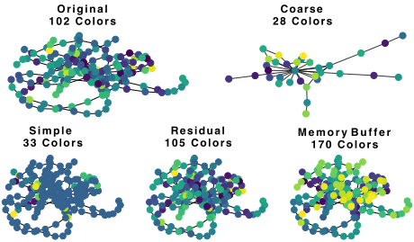
Hierarchical Graph Neural Networks (HGNNs) aim to address this challenge by constructing progressively coarse graph representations, where groups of nodes are pooled into higher-level super nodes to expose large-scale trends [Yang et al., 2021]. In principle, these global patterns should guide the evolution of the original node-level representations during forecasting. However, as illustrated in Figure 1, we find that existing HGNNs fail to deliver this guidance effectively. The weaker coloring indicates less discovery of spatio-temporal trends, negatively affecting downstream forecasting performance [Jin et al., 2025; Cai et al., 2024; Ye et al., 2022]. We identify an unformalized failure mode, downward memory loss, in which global features learned at coarse levels rapidly diminish when propagated back to the fine-grained, node-level representations. As a result, HGNNs effectively revert to behaving similarly to single-scale GNNs, with global information exerting little influence on final predictions.
Despite the widespread use of HGNNs, this degradation phenomenon has not been formally studied. We demonstrate that common design choices, such as residual connections [Oskarsson et al., 2024], are insufficient in resolving the issue. While residual connections are commonly used in HGNNs to re-inject global trends into node-level representations, they operate in the same information stream as the projecting and embedding maps. As a result, global features are immediately remixed, remaining subject to subsequent information loss. Thus, residual connections cannot prevent downward memory loss identified in this work. Our analysis reveals the underlying cause of this information decay: the linearity of the coarse-to-fine transition mappings used in existing HGNNs. These linear mappings inherently oversmooth global features, erasing the distinctions needed for reliable global-to-local alignment. We also show that post-processing via a nonlinear map mitigates this oversmoothing effect. To the best of our knowledge, this is the first theoretical analysis linking linear hierarchical decoding to oversmoothing in HGNN forecasters.
To address these limitations, we propose HiGFlow, a new HGNN forecaster that preserves multiscale coherence across all levels of the hierarchy. Instead of allowing global information to fade as it returns to the node level, HiGFlow updates an isolated memory variable by jointly using signals from both coarse and fine representations, preventing the forgetting that would otherwise occur in the main branch. This information retention enables consistent information flow across scales, allowing node-level predictions to remain aligned with global temporal drivers. We demonstrate theoretically that utilizing the memory buffer facilitates the enhancement of spatiotemporal trend discovery. Additionally, we show that residual connections are limited in uncovering these trends, as evident by the comparison made in Figure 1. Table 1 summarizes the benefits of the memory buffer over residual (res), no retention (ret) and transformer attention (trans) methods.
Extensive experiments across standard multivariate forecasting benchmarks demonstrate that HiGFlow achieves state-of-the-art performance. The model consistently outperforms graph-based [Yi et al., 2024a] and transformer-based forecasters [Wang et al., 2025a; Nie et al., 2023; Liu et al., 2024], and delivers substantial gains over state-of-theart multiscale methods [Hu et al., 2025; Wang et al., 2025a; Wang et al., 2025b]. HiGFlow consistently reduces MAE and RMSE over the state-of-the-art by substantial margins, confirming the importance of preserving global-scale information when forecasting from fine-grained, node-level inputs.
Our contributions are as follows: (1) We define and formalize downward memory loss, showing that global features learned at coarse levels fail to effectively influence nodelevel predictions in existing HGNNs. (2) We provide the first formal connection between linear coarse-to-fine transitions and oversmoothing, explaining the structural origin of global information decay. (3) We propose HiGFlow, a memorybuffered enhanced HGNN with nonlinear, bidirectional coupling that preserves multiscale coherence from coarse to node-level representations. (4) We achieve new state-of-theart forecasting accuracy across diverse benchmarks, demonstrating the practical value of maintaining global information throughout hierarchical decoding.
| Methods Property | HGNN No Ret. | Trans. Attn Mixing | HGNN Residual | HiGFlow Memory |
|---|---|---|---|---|
| Global Retention | × | × | ✓ | ✓ |
| Coarse Remixing | ∼ | × | ✓ | ✓ |
| Trend Discovery | × | ∼ | ∼ | ✓ |
| Global →Local | ∼ | × | ∼ | ✓ |
| Joint Mixing | × | ∼ | × | ✓ |
2 RelatedWork
Multivariate Forecasting with Graph Neural Networks. Through their ability to directly model ground truth topology across a wealth of domains, GNNs have emerged as a powerful paradigm across multivariate forecasting tasks [Lam et al., 2023; Lan et al., 2022; Zhang et al., 2021; Bauer et al., 2015], which contain strongly interconnected spatio-temporal relationships. Recent models, such as SFGDE [Cui et al., 2025] or HDS [Yan et al., 2024], incorporate state feedback to prevent oversmoothing, enabling the stacking of an arbitrary number of layers without performance degradation. Even without a ground-truth graph available, several works have demonstrated that a descriptive topology is learnable from domain-specific processes latent within the input buffer via a time series to graph embedding. For instance, [Wu et al., 2023b] optimize topology within a latent space, which is shown to be equivalent to optimizing a measure for global consistency. Other works, such as those by [Yi et al., 2024a] and [Cao et al., 2020], utilize cross-attention to learn the topology. DGraFormer [Yan et al., 2025] learns a sequence of relatively small spatial graphs through discretizing the series into various windows, removing noise while improving computational efficiency. However, in many cases, a ground truth graph exists, such as in traffic flow prediction [Lan et al., 2022], where traffic networks overlay rich spatial contexts over observed samples. In our work, we broaden the vision of GNNs to view these contexts at multiple scales.
Hierarchical Methods for Multiscale Modeling. Though strictly edge-based GNNs are effective within the bounds of capturing interactions at a single resolution, they are unable to capture global spatio-temporal trends, which are integral to the development of a multivariate time series. Recent non-graph forecasters such as FilterTS, AMD, and TimeMixer++ [Hu et al., 2025; Wang et al., 2025a; Wang et al., 2025b] achieve state-of-the-art multivariate forecasting by decomposing temporal signals into multiscale components and adaptively mixing temporal and channel-wise patterns. However, they do not directly learn relationships at multiple spatio-temporal scales, which allows for valuable insights into time series dynamics. Hierarchical GNNs (HGNNs) [Oskarsson et al., 2024; Cini et al., 2023; Yang et al., 2021; Guo et al., 2021] address the structural side of the multiscale modeling challenge, learning multiscale representations by integrating coarse features and graphs into forecasts. Beyond regularly sampled data, HiPatch [Luo et al., 2025] hierarchically couples patches to enhance multiscale correlation for sparsely sampled data. Applied works such as [Oskarsson et al., 2024] propose a probabilistic ensemble method using an HGNN with residual connections. [Cini et al., 2023] find assignment matrices via clustering methods to build the hierarchy based on linear, first-order relationships. We propose in our work a memory-buffer that nonlinearly adjusts fine-grain features through preserving coarse representations, provably enhancing the discovery of trends while avoiding oversmoothing arising from linear transitions.
3 Preliminaries
Forecasting. We define a time series at time t as a finegrained signal x(t; T ) ∈ RN×T , representing N spatial variables over a sliding window of length T covering the interval [t, t + T]. Given an input signal x(t; Tin) with buffer size Tin, the forecasting task predicts the subsequent signal over Tout time steps, denoted by x(t + Tin; Tout). We denote the T-dimensional row vector corresponding to variable i as xi(t; T ). For brevity, we write x(t) = x(t; 0) ∈ RN×1 .
Timeseries to Graph Embeddings. We enrich the descriptiveness of the feature space by embedding our input signal onto a hidden dimension of size D with weight vector we ∈ RD and activation function σ:
where h(t; Tin) ∈ RN×Tin×D . [Cao et al., 2020] and [Yi et al., 2024a] learn the underlying spatio-temporal interactions within h(t; Tin) via time series to graph embeddings. Here, we consider each (i, t) ∈ [1,N] × [1, Tin] to be a node within the vertex set of a graph, and find edge-weights that capture association between spatio-temporal variables via self-attention, where edge weights A are proportional to h(t; Tin) · h(t; Tin)T . See Appendix C for pseudo code of this algorithm.
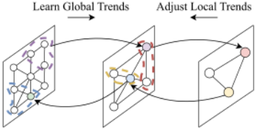
Hierarchical Graph Neural Networks. HGNNs model interactions between multiscale trends, thereby enhancing insight into underlying time series dynamics. To learn global trends, as illustrated in Figure 2, HGNNs cluster a fine-grain graph Gi to create a coarse graph Gi+1, mapping features hu,i(t) onto hv,i+1(t) for u ∈ Cv,i+1, the vth cluster on Gi. Conversely, HGNNs adjust these local features on Gi by projecting (lifting) onto the features of Gi+1. We formalize the feature coarsening and projecting operations of HGNNs in the following definition:
Definition 1 (Transition Function). A transition function F : X(Gn) → X(Gm) maps features on Gn to Gm:
where Cj,n is the jth cluster of Gn. When n = i + 1 and m = i, then F is a lifting map. Conversely, when n = i and m = i + 1, then is a F embedding map.
When embedding, the features of the cluster are aggregated to reduce its dimension. In contrast, lifting maps invert this process, copying the feature to match the size of the cluster. To separate these two concepts, we write the embedded and lifted features at height i as h:,i(t) and u:,i(t). We also write the collection of all clusters on Gi, for any i, as Ci.
4 Hierarchical Graph FlowNetwork
We formalize how HiGFlow improves the capture of spatiotemporal trends. Section 4.1 elaborates on how the memory buffer preserves global trends that would otherwise be lost when using residual connections. Section 4.2 proves the effectiveness of HiGFlow's transition maps, while Section 4.3 provides the architectural details of these components.
4.1 Storing Global Trends in aMemory Buffer
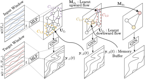
The downward pass in HGNNs constructs a multiscale view of spatiotemporal relationships by adjusting local trends to better align with global ones. Accordingly, it is key to their downstream performance. However, even if HGNNs effectively learn global trends, they do not necessarily integrate these into fine-grained features when rolling out over the forecast horizon. In Figure 3, we illustrate how HiGFlow improves on the process of producing forecasts. Critically, while adjusting local patterns, the memory buffer also keeps track of previously seen global trends, allowing for their continued use during the local feature refinement process.
Functional Description. Here we provide a formulation of the memory buffer. To initialize then update the memory buffer contents, we incorporate both u:,i(t) and h:,i(t), the lifting and embedding tensors of Gi, into the GNN Dδi :
Section 4.2 provides further details on how u:,i(t) is derived. By storing observed trends within a separate variable, y:,i(t), which acts as a memory buffer, we set aside storage for trend preservation, thereby enhancing the representational capacity of HiGFlow beyond that of existing HGNNs. We formally show this claim in Theorem 1.
Enhanced Expressivity. We show in Theorem 1 the effect of the memory buffer on preserving global trends, shown via graph coloring. A more intricate coloring allows for graph structures, which describe spatio-temporal trends, to be differentiated when they would otherwise be treated as the same. In this way, coloring acts as a necessary condition on trend discovery. Theorem 1 also shows that coloring is stable with respect to hierarchical depth, i.e. the memory buffer preserves global trends across hierarchical levels:
Theorem 1. An HGNN implementing the memory buffer in Equation 3 in a K-level hierarchy omits the memory enhanced hash function g1(x1, . . . , xK) = h2(x1, g2(x2, . . . , xK)), where any hi, for 1 ≤ i ≤ K is an injective hash function. Then, for the consequent graph coloring X t k (G), where k is the number of recursions:
In this context, the coloring X t k (G1) is the set of colors over G1 in terms of the 1-WL hash-functions h1, . . . , hK [Xu et al., 2019], where the colors act as surrogates for graph features. Theorem 1 serves as a weak but general condition that is necessary for trend discovery.
Given Theorem 1 applies to HiGFlow, an HGNN equipped with a memory buffer, a question of critical importance would be whether a similar statement applies when building an HGNN with residual connections. We show in Lemma 1 that this is not the case, specifically because residual connections do not preserve the injectivity property, which leads to distinct trends becoming homogeneous in model vision. In practice, the result asserts that topological indistinguishability increases as a result of feature similarity.
Lemma 1. Suppose we have an HGNN equipped with residual connections in its architecture. Then the induced hash function g1(xk, . . . , xK) = h1(x1) + g2(x2, . . . , xK) is not injective, even if all hk are.
4.2 Deriving Effective Transition Functions
We present theoretical results regarding the loss in distinctness of global trends that result from transition function linearity, using the Dirichlet Energy as a measure for graph-wide similarity.
Definition 2 (Dirichlet Energy). The Dirichlet energy measures the similarity between feature vectors within Gi, for some level i, and is normalized via the inverse degree matrix:
where du,i is the degree of node u in Gi.
In principle, our results originate from the notion that there is an optimal range the Dirichlet Energy occupies, which is strongly tied to the homogeneity of the original graph, G1, which we assume to be ideal. Decreasing this metric through coarsening indicates that dissimilar trends have become less distinct [Wu et al., 2023c; Rusch et al., 2023; Chen et al., 2020], whereas an increase in the metric suggests the presence of spurious correlation. In Theorem 2, we show that not post-processing the coupling between Gi and Gi+1 decrease the Dirichlet Energy:
Theorem 2. Suppose Ai and Ai+1 are the adjacency matrices of Gi and Gi+1, for some i, and Pi↦→i+1 ∈ {0, 1}Ni×Ni+1 is a assignment matrix that linearly couples via the relation h:,i+1(t) = Pi↦→i+1 · h:,i(t). Then the total Dirichlet energy contracts when between Gi and Gi+1 in either direction.
Next, we expand on Theorem 2 with Theorem 3, which suggests that applying a nonlinear transformation, after coupling with Pi↦→i+1 · hi(t) or Pi+1↦→i · hi+1(t), mitigates the severity of energy contraction:
Theorem 3. Assume the same conditions as in Theorem 2. Additionally, consider the power-series expansion with B non-zero power-series coefficients ωb of some function f: f(h) = ∑∞b=1 ωb ·hb = ∑Bb=1 ωb ·hb . If h and f(h) are normalized such that ∥h∥2 ≤ 1 and ∥f(h)∥2 ≤ 1, then neither transition function M = f ◦ Pi↦→i+1 nor U = f ◦ Pi+1↦→i exhibits energy contraction as B ↦→ ∞.
Intuitively, Theorem 3 holds since relatively small differences in the features h:,i(t) and h:,i+1(t) are more greatly emphasized. Theorem and Lemma 1 suggest that the memory buffer is more nonlinear than using Residual connections.
4.3 TransitionMap Architecture
We provide a detailed explanation of how HiGFlow learns global trends and subsequently creates new local patterns.
Learning Global Trends. We learn the latent global relationships described within Gi through the topologies of its subgraphs Cj,i ∈ Ci. We aggregate the features of the cluster hu,i(t), for u ∈ V (Cj,i). Additionally, we also aggregate the topology of Gi by assigning an edge between u, v ∈ V (Gi+1) if an edge exists between nodes of Cu,i and Cv,i. Both of these operations are easily achievable through multiplying by the incident matrix Pi↦→i+1 ∈ {0, 1}Ni+1×Ni , that is h:,i(t) ↦→ Pi↦→i+1 · h:,i(t), which locally reduces to a summation over the features of each Cj,i:
Furthermore, the topology of Gi is aggregated into the adjacency matrix of Gi+1, Ai+1 = D-1 i+1 · Pi↦→i+1 · Ai, where we normalize via the new adjacency matrix with degree matrix Di+1 ∈ RNi+1×Ni+1 , which satisfies Di,j = |Ci,j |.
| Models | Traffic | Electricity | PEMS03 | PEMS04 | PEMS07 | PEMS08 | ||||||
|---|---|---|---|---|---|---|---|---|---|---|---|---|
| MAE | RMSE | MAE | RMSE | MAE | RMSE | MAE | RMSE | MAE | RMSE | MAE | RMSE | |
| FourierGNN [Yi et al., 2024a] | 0.278 | 0.551 | 0.266 | 0.398 | 0.146 | 0.215 | 0.164 | 0.251 | 0.139 | 0.214 | 0.152 | 0.227 |
| FreTS [Yi et al., 2024b] | 0.320 | 0.613 | 0.334 | 0.501 | 0.154 | 0.225 | 0.170 | 0.259 | 0.172 | 0.261 | 0.147 | 0.224 |
| DLinear [Zeng et al., 2023] | 0.465 | 0.774 | 0.381 | 0.549 | 0.159 | 0.232 | 0.176 | 0.266 | 0.152 | 0.231 | 0.165 | 0.243 |
| Autoformer [Wu et al., 2021] | 0.345 | 0.589 | 0.277 | 0.395 | 0.150 | 0.221 | 0.164 | 0.253 | 0.143 | 0.220 | 0.151 | 0.225 |
| Informer [Zhou et al., 2021] | 0.312 | 0.608 | 0.265 | 0.374 | 0.180 | 0.294 | 0.185 | 0.295 | 0.209 | 0.365 | 0.177 | 0.265 |
| NS-Transformer [Wu et al., 2023a] | 0.304 | 0.589 | 0.247 | 0.383 | 0.143 | 0.218 | 0.162 | 0.259 | 0.140 | 0.224 | 0.153 | 0.237 |
| FEDformer [Zhou et al., 2022] | 0.330 | 0.501 | 0.278 | 0.393 | 0.140 | 0.207 | 0.159 | 0.247 | 0.138 | 0.214 | 0.153 | 0.231 |
| TimesNet [Wu et al., 2023a] | 0.315 | 0.594 | 0.218 | 0.325 | 0.143 | 0.210 | 0.160 | 0.246 | 0.135 | 0.210 | 0.146 | 0.218 |
| iFlashformer [Liu et al., 2024] | 0.283 | 0.557 | 0.288 | 0.415 | 0.143 | 0.214 | 0.163 | 0.255 | 0.141 | 0.218 | 0.148 | 0.226 |
| iTransformer [Liu et al., 2024] | 0.298 | 0.600 | 0.303 | 0.467 | 0.145 | 0.216 | 0.165 | 0.256 | 0.139 | 0.217 | 0.153 | 0.231 |
| FilterTS [Wang et al., 2025b] | 0.407 | 0.704 | 0.309 | 0.467 | 0.150 | 0.221 | 0.169 | 0.260 | 0.144 | 0.221 | 0.159 | 0.237 |
| TimeMixer++ [Wang et al., 2025a] | 0.250 | 0.504 | 0.217 | 0.323 | 0.145 | 0.212 | 0.160 | 0.246 | 0.138 | 0.212 | 0.148 | 0.221 |
| AMD [Hu et al., 2025] | 0.301 | 0.582 | 0.293 | 0.435 | 0.166 | 0.237 | 0.175 | 0.258 | 0.158 | 0.230 | 0.174 | 0.254 |
| HiGFlow(1) | 0.305 | 0.593 | 0.347 | 0.524 | 0.151 | 0.222 | 0.172 | 0.261 | 0.149 | 0.224 | 0.158 | 0.234 |
| HiGFlow | 0.225 | 0.484 | 0.215 | 0.324 | 0.139 | 0.210 | 0.153 | 0.238 | 0.131 | 0.204 | 0.145 | 0.217 |
| Gain vs best baseline (%↓) | +10.0% | +3.4% | +0.9% | -0.3% | +0.7% | -1.4% | +3.8% | +3.3% | +3.0% | +2.9% | +0.7% | +0.5% |
According to Theorem 2 and 3, using the linear coupling Pi↦→i+1 as a transition function reduces the distinctiveness of global relationships. We therefore post-process with a neural network Mϕi :
Here, we embed contextual information via the node index vector vi+1 = (1, . . . ,Ni+1)T and a learnable matrix We i+1 ∈ RNi+1×D projecting onto a D dimensional vector.
Projecting Global Trends to Local Trends. In Section 4.1, we discussed the role of u:,i(t) as a means of incorporating learnt global trends within the memory buffer mechanism. We now provide additional details on how features u:,i(t) are derived from global trends within h:,i+1(t).
In particular, the functional form remains consistent with that of embeddings from Gi to Gi+1. The only difference is that the assignment matrix Pi+1↦→i, which is equal to P T i↦→i+1 , is now a one-to-many mapping. The initial projection, for instance, is given by u:,i(t) = Pi+1↦→i · y:,i+1(t), copying the features of each node j ∈ V (Gi+1) to every q ∈ V (Cj,i):
We follow Theorem 2 and 3, as we discussed during embeddings, to post-process the result with network Uξi :
In the above equation, vi = (1, . . . ,Ni)T denotes node indices of Gi, andWli ∈ RNi×D , their learnable linear embedding that projects them onto a D dimensional space.
5 Experiments
HiGFlow introduces a scale-adaptive memory buffer to mitigate downward memory loss. We evaluate HiGFlow against state-of-the-art forecasting models on eight realworld datasets, and further evaluate various internal behaviors, addressing the following research questions:
- RQ1. Is HiGFlow able to forecast short lead times effectively with a limited input window? How does its performance compare to state-of-the-art models?
- RQ2. Given that the memory buffer theoretically improves on residual connections for HGNNs, what is the difference in performance between these and HiGFlow over forecasting benchmarks?
- RQ3. To what extent do HiGFlow's transition functions reduce information loss? How does their linearity affect downstream accuracy, and do the distinctiveness of learnt patterns align with our theoretical claims?
To address these questions, we complement our baseline comparisons with experiments that isolate the effect of transition-map linearity, HiGFlow's downstream performance, and Dirichlet energy. Appendix B provides additional experiments, including sensitivity HiGFlow to the clustering factor and use of node embeddings, computational training cost, and further comparisons over more benchmarks.
5.1 Experimental Set Up
Datasets. We evaluate on real-world forecasting datasets: Electricity and Traffic, which use a time-series-to-graph embedding in our pipeline, and PEMS-Bay, which provides a graph encoding physical relationships. Appendix B reports additional results on ECG, Solar, ETTh1, and ETTm1 [Wu et al., 2022], which exhibit strong temporal correlations. For all datasets, we use a 60%/20%/20% split for training/validation/testing and apply z-score normalization during both training and testing.
Baselines. We compare HiGFlow with state-of-the-art multiscale forecasters, including TimeMixer++ [Wang et al., 2025a], AMD [Hu et al., 2025], FilterTS [Wang et al.,
2025b]. We also include Autoformer [Wu et al., 2022] and DLinear [Zeng et al., 2023] as strong multiscale baselines. In addition, we evaluate frequency-domain methods, namely FourierGNN [Yi et al., 2024a], FreTS [Yi et al., 2024b], and FEDformer [Zhou et al., 2022]. We further include transformer-based forecasters, including iTransformer and iFlashformer [Liu et al., 2024], TimesNet [Wu et al., 2023a], Informer [Zhou et al., 2021] and NS-Transformer [Wu et al., 2023a]. We use HiGFlow(1) to denote the singlelevel model (height 1), and HiGFlow to denote the two-level model (height 2). All baselines were run with their original optimal parameter settings.
Experiment Settings. We run all experiments on a single NVIDIA A100 GPU. We train using mean squared error with the RMSProp optimizer, a dropout rate of 0.6, and an initial learning rate of 5 × 10⁻⁴ that decays by a factor of 0.7 every 5 epochs. We train for 50 epochs and report Mean Absolute Error (MAE) and Root Mean Squared Error (RMSE). Unless otherwise stated, we evaluate short-term forecasting horizons Tout ∈ {3, 6, 9, 12} and fix the input buffer length to Tin = 12. These settings follow prior short-term forecasting work [Cui et al., 2025; Wang et al., 2025a; Cao et al., 2020; Yi et al., 2024a]. We construct a hierarchy of height 2 by clustering 0.9 percent of all nodes in the base graph, which we verify in Appendix B to always be the optimal choice. HiGFlow uses the spectral convolution from [Cao et al., 2020] as the memory-buffer GNN Dδ .
5.2 Evaluation
Performance over Traffic and Electricity (RQ1). In Table 2, we evaluate HiGFlow on Traffic and Electricity against the baselines listed in Section 5.1 over a short-term forecasting horizon of 3. In these settings, HiGFlow encodes the timeseries onto a graph, meaning spatiotemporal relationships must be inferred. HiGFlow outperforms TimeMixer++, AMD, and FilterTS over Traffic, achieving substantial gains of at least 10% in MAE and 4% in RMSE. Over Electricity, TimeMixer++, and HiGFlow are comparable. In comparison to the remaining transformer and GNN baselines, HiGFlow demonstrates substantial improvement. Furthermore, given the large error reduction, it is clear when comparing HiGFlow(1) and HiGFlow that GNN forecasters benefit frommodeling local trends at a coarse scale.
Performance over PEMS (RQ1). We further evaluate in Table 2 HiGFlow on the PEMS benchmarks. These datasets use a real road-network graph that provides physical structure, providing a reliable basis for GNN forecasting methods. HiGFlow obtains the lowest MAE and RMSE on most datasets, obtaining the second-best RMSE only on PEMS03. TimesNet, FEDformer, and TimeMixer++ emerge as the strongest baselines, frequently obtaining the secondlowest error metrics. HiGFlow reduces MAE by 0.7-3.8% and RMSE by 0.5-3.3% over these three models. Comparing against other strong baselines, HiGFlow further scores an average reduction of 5.6% and 5.5% against iTransformer, 5.5% and 4.1% against FourierGNN, and 8.7% and 7.4% against FilterTS in terms of MAE and RMSE, respectively. Overall, these results indicate that HiGFlow generalizes across both scenarios, when working with learned graph embeddings (Traffic/Electricity) and when forecasting with groundtruth graphs (PEMS). We provide additional experiments over temporal datasets in Appendix B.
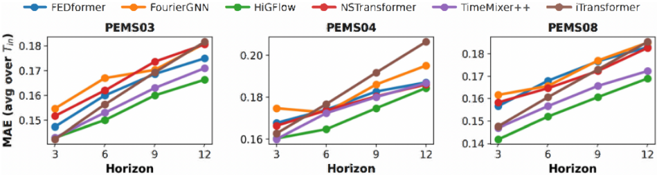
Evaluating Performance when Increasing Forecast Horizon and Buffer Size (RQ1). We broaden our evaluation of HiGFlow on short-term forecasting by varying both the prediction horizon and the input buffer size. We thereby extend our previous experiments in Figure 4, averaging the MAE over input buffer sizes of 12, 24 and 48, comparing with baselines that have strong long and short term forecasting capabilities. Full result tables for each buffer size are available in Appendix B. On average, HiGFlow attains, or ties for, the best performance in 10 of 12 cases, often by substantial margins, showing that performance is consistent across variations of both horizons and input buffer sizes.
Performance Difference between Memory Buffer and Residual Connections (RQ2). We expand on the comparison made in Figure 1 by isolating the impact of the memory buffer on performance, and investigate the outcome of using alternative residual connection-based architectures instead. We compare HiGFlow with Simple, an HGNN with no global retention, Residual, a HGNN that adds residual connections between levels, and Hybrid, which uses both the memory buffer and residual connections. Table 3 shows the outcomes of our experiments. HiGFlow outperforms alternative architectures across all benchmarks. Furthermore, HiGFlow achieves substantial gains regardless of the use of graph embeddings. This validates our memory buffer as a more practical method for HGNNs than that of residual connections. Through comparing Residual and Hybrid with Simple, we further observe that they enhance performance on 4 of 6 datasets. This suggests that memory retention mechanisms are generally an important component of HGNNs, although the effective use of coarse features significantly enhances their capacity.
| Model | Traffic | Electricity | PEMS03 | PEMS04 | PEMS07 | PEMS08 | ||||||
|---|---|---|---|---|---|---|---|---|---|---|---|---|
| MAE | RMSE | MAE | RMSE | MAE | RMSE | MAE | RMSE | MAE | RMSE | MAE | RMSE | |
| Simple | 0.673 | 1.010 | 0.628 | 0.812 | 0.151 | 0.223 | 0.165 | 0.251 | 0.139 | 0.213 | 0.152 | 0.227 |
| Residual | 0.291 | 0.566 | 0.285 | 0.418 | 0.150 | 0.221 | 0.174 | 0.264 | 0.154 | 0.230 | 0.146 | 0.219 |
| Hybrid | 0.266 | 0.535 | 0.254 | 0.383 | 0.154 | 0.229 | 0.167 | 0.251 | 0.149 | 0.221 | 0.154 | 0.228 |
| HiGFlow | 0.225 | 0.484 | 0.215 | 0.324 | 0.139 | 0.210 | 0.153 | 0.238 | 0.131 | 0.204 | 0.145 | 0.217 |
| Gain(%) | +15.41% | +9.53% | +15.35% | +15.40% | +7.33% | +4.98% | +7.27% | +5.18% | +5.76% | +4.23% | +0.68% | +0.91% |
Overhead fromMemory Buffer (RQ2). We analyze the overhead introduced by the memory buffer over existing information retention methods for HGNNs. Table 4 summarizes runtimes per epoch over PEMS08 while the input buffer size increases. We observe that Residual, by running a GNN only on the coarse features, often achieves the lowest runtime, while HiGFlow marginally achieves the second-lowest runtime. The combination of memory buffer and residual methods in Hybrid slightly increases the runtime. Overall, it appears that HGNNs generally scale poorly with respect to input buffer size when using a hypergraph, which scales the size of the graph by order N · Tin. In practice, embedding the temporal dimension and using higher coarsening factors would further reduce the overhead of HGNNs over edge-based GNN models. In Appendix B, we compare the runtime of HiGFlow and baseline methods.
| Input Buffer Size | ||||
|---|---|---|---|---|
| Model | 12 | 24 | 36 | 48 |
| HiGFlow | 11.0±0.1 | 18.8 ±1.0 | 31.9±0.2 | 41.0±0.2 |
| Residual | 8.8±0.1 | 14.0±0.1 | 23.3±0.1 | 29.3±0.2 |
| Hybrid | 11.0 ±0.1 | 18.6 ±0.4 | 32.1±0.1 | 41.3±0.1 |
| Simple | 11.1±0.1 | 18.4 ±0.2 | 32.1±0.2 | 41.2±0.1 |
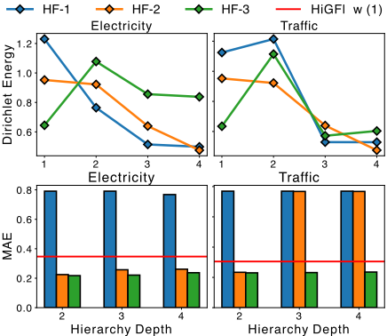
Hierarchical Height and Transition Capacity (RQ3). We empirically assess the extent to which Theorems 2 and 3 manifest in practice. We vary the capacity of HiGFlow's transition function using three variants: HF-1, a linear map implemented via matrix multiplication; HF-2, a one-hiddenlayer MLP; and HF-3, a two-hidden-layer MLP. For Traffic and Electricity, we report both the level-wise Dirichlet Energy of a height four HiGFlow and the final MAE incurred for HiGFlow variants of varying heights. Nonlinear transitions outperform linear mappings, with HF-1 exhibiting a significant error over both datasets. Furthermore, the performance of HF-2 declines significantly at depths exceeding 2 over Traffic, indicating a severe collapse in modeling capacity. Patterns in the Dirichlet Energy plot suggest why: the linear transition typically yields a near-monotone decrease in energy as depth increases, an observation aligning well with Theorem 2. In contrast, HF-2 and HF-3 reduce energy either more gradually or not in a consistently monotone manner, evidencing Theorem 3. These results support the claim that nonlinear transitions mitigate the loss of coarse features when modeling intricate spatiotemporal trends.
6 Conclusion
We address downward memory loss in hierarchical GNNs (HGNNs), where learned coarse features exert diminishing influence on local representations. We demonstrate that trend distinctiveness is degraded under linear transition maps and that nonlinear maps mitigate this effect. Although residual connections reduce forgetting, they yield weaker theoretical guarantees and inferior empirical performance. To overcome these limitations, we propose HiGFlow, an HGNN that stores global trends in a dedicated memory buffer. This buffer captures a broader range of spatiotemporal trends. We validate our theory in real-world experiments and find close agreement between predicted and observed behavior. Finally, HiGFlow achieves state-of-the-art performance in short-term forecasting across various benchmarks.
Acknowledgments
This research is supported by MBIE Strategic Science Investment Fund (SSIF) Data Science platform - Time-Evolving Data Science / Artificial Intelligence for Advanced Open Environmental Science (UOWX1910).
@inproceedings{ijcai2026p462,
  title     = {Addressing Downward Memory Loss in Hierarchical GNN Forecasters Through Memory-Buffered Decoding},
  author    = {Bailie, Thomas and Mukkavilli, S. Karthik and Vetrova, Varvara and Koh, Yun Sing},
  booktitle = {Proceedings of the Thirty-Fifth International Joint Conference on
               Artificial Intelligence, {IJCAI-26}},
  publisher = {International Joint Conferences on Artificial Intelligence Organization},
  editor    = {Diego Calvanese},
  pages     = {4152--4160},
  year      = {2026},
  month     = {8},
  note      = {Main Track},
  doi       = {10.24963/ijcai.2026/462},
  url       = {https://doi.org/10.24963/ijcai.2026/462},
}
TY - CPAPER TI - Addressing Downward Memory Loss in Hierarchical GNN Forecasters Through Memory-Buffered Decoding AU - Bailie, Thomas AU - Mukkavilli, S. Karthik AU - Vetrova, Varvara AU - Koh, Yun Sing T2 - Proceedings of the Thirty-Fifth International Joint Conference on Artificial Intelligence, IJCAI-26 PB - International Joint Conferences on Artificial Intelligence Organization PY - 2026 SP - 4152 EP - 4160 DO - 10.24963/ijcai.2026/462 UR - https://doi.org/10.24963/ijcai.2026/462 ER -Copied
Machine-readable versions of this paper, for tools and AI agents:





