
State Feedback Enhanced Graph Differential Equations for Multivariate Time Series Forecasting
Proceedings of the Thirty-Fourth International Joint Conference on Artificial Intelligence. Main Track. Pages 7374-7382.
https://doi.org/10.24963/ijcai.2025/820
Keywords
- Machine Learning: ML: Time series and data streams
- Data Mining: DM: Mining spatial and/or temporal data
- Multidisciplinary Topics and Applications: MTA: Web and social networks
Abstract
Multivariate time series forecasting holds significant theoretical and practical importance in various fields, including web analytics and transportation. Recently, graph neural networks and graph differential equations have shown exceptional capabilities in modeling spatio-temporal features. However, existing methods often suffer from over-smoothing, hindering real-world problem-solving. In this work, we analyze the graph propagation process as a dynamical system and propose a novel feedback mechanism to enhance representation power, adaptively adjusting the representations to align with desired performance outcomes, thereby fundamentally mitigating the issue of over-smoothing. Moreover, we introduce an effective multivariate time series forecasting model called SF-GDE, based on the proposed graph propagation with the feedback mechanism. Intensive experiments are conducted on three real-world datasets from diverse fields. Results show that SF-GDE outperforms the state of the arts, and the feedback mechanism can serve as a universal booster to improve performance for graph propagation models.
- [Abramowitz and Stegun, 1964] Milton Abramowitz and Irene A Stegun. Handbook of mathematical functions with formulas, graphs, and mathematical tables. US Government printing office, 1964.
- [Bai et al., 2020] Lei Bai, Lina Yao, Can Li, Xianzhi Wang, and Can Wang. Adaptive graph convolutional recurrent network for traffic forecasting. In NeurIPS, pages 1-16, 2020.
- [Barzel and Barabási, 2013] B. Barzel and A-L Barabási. Universality in network dynamics. Nature Physics, 9(10):673-681, 2013.
- [Berberich et al., 2020] Julian Berberich, Anne Koch, Carsten W Scherer, and Frank Allgöwer. Robust data- driven state-feedback design. In ACC, pages 1532-1538. IEEE, 2020.
- [Box et al., 2015] George EP Box, Gwilym M Jenkins, Gre- gory C Reinsel, and Greta M Ljung. Time Series Analysis: Forecasting and Control. John Wiley & Sons, 2015.
- [Bruna et al., 2014] Joan Bruna, Wojciech Zaremba, Arthur Szlam, and Yann LeCun. Spectral networks and deep lo- cally connected networks on graphs. In ICLR, pages 1-14, 2014.
- [Casado-Vara et al., 2021] Roberto Casado-Vara, Angel Martin del Rey, Daniel Pérez-Palau, Luis de-la Fuente- Valentín, and Juan M Corchado. Web traffic time series forecasting using lstm neural networks with distributed asynchronous training. Mathematics, 9(4):421, 2021.
- [Chen et al., 2018] Ricky TQ Chen, Yulia Rubanova, Jesse Bettencourt, and David Duvenaud. Neural ordinary differ- ential equations. In NeurIPS, pages 6572-6583, 2018.
- [Chen et al., 2020] Deli Chen, Yankai Lin, Wei Li, Peng Li, Jie Zhou, and Xu Sun. Measuring and relieving the over- smoothing problem for graph neural networks from the topological view. In AAAI, pages 3438-3445, 2020.
- [Chen et al., 2024] Peng Chen, Yingying ZHANG, Yunyao Cheng, Yang Shu, Yihang Wang, Qingsong Wen, Bin Yang, and Chenjuan Guo. Pathformer: Multi-scale trans- formers with adaptive pathways for time series forecast- ing. In ICLR, 2024.
- [Cui et al., 2024] Jiaxu Cui, Qipeng Wang, Bingyi Sun, Jim- ing Liu, and Bo Yang. Learning continuous network emerging dynamics from scarce observations via data- adaptive stochastic processes. Science China Information Sciences, 67(12):222206, 2024.
- [Cunningham, 1962] W. J. Cunningham. An introduction to lyapunov's second method. Transactions of the American Institute of Electrical Engineers, Part II: Applications and Industry, 80(6):325-332, 1962.
- [Defferrard et al., 2016] Michaël Defferrard, Xavier Bres- son, and Pierre Vandergheynst. Convolutional neural net- works on graphs with fast localized spectral filtering. In NeurIPS, pages 3844-3852, 2016.
- [Dong et al., 2021] Shi Dong, Ping Wang, and Khushnood Abbas. A survey on deep learning and its applications. Computer Science Review, 40:100379, 2021.
- [Erichson et al., 2019] N Benjamin Erichson, Michael Muehlebach, and Michael W Mahoney. Physics-informed autoencoders for lyapunov-stable fluid flow prediction. In NeurIPS, pages 1-6, 2019.
- [Fang et al., 2021] Zheng Fang, Qingqing Long, Guojie Song, and Kunqing Xie. Spatial-temporal graph ode net- works for traffic flow forecasting. In ACM SIGKDD, pages 364-373, 2021.
- [Gao et al., 2022] Junyi Gao, Cao Xiao, Lucas M Glass, and Jimeng Sun. Popnet: Real-time population-level disease prediction with data latency. In WWW, pages 2552-2562, 2022.
- [Garza and Mergenthaler-Canseco, 2023] Azul Garza and Max Mergenthaler-Canseco. Timegpt-1. arXiv:2310.03589, 2023.
- [Gopal, 1993] Madan Gopal. Modern control system theory. New Age International, 1993.
- [Gravina et al., 2024] Alessio Gravina, Daniele Zambon, Davide Bacciu, and Cesare Alippi. Temporal graph odes for irregularly-sampled time series. In IJCAI, 2024. IJCAI
- [Greff et al., 2017] Klaus Greff, Rupesh K. Srivastava, Jan Koutník, Bas R. Steunebrink, and Jürgen Schmidhuber. LSTM: A search space odyssey. IEEE Transactions on Neural Networks and Learning Systems, 28(10):2222- 2232, 2017.
- [Houde and Nagarajan, 2011] John F Houde and Srikantan S Nagarajan. Speech production as state feedback control. Frontiers in human neuroscience, 5:82, 2011.
- [Hu et al., 2023] Junfeng Hu, Yuxuan Liang, Zhencheng Fan, Hongyang Chen, Yu Zheng, and Roger Zimmermann. Graph neural processes for spatio-temporal extrapolation. In ACM SIGKDD, 2023.
- [Huang et al., 2020] Rongzhou Huang, Chuyin Huang, Yubao Liu, Genan Dai, and Weiyang Kong. LSGCN: Long short-term traffic prediction with graph convolu- tional networks. In IJCAI, pages 2355-2361, 2020. IJCAI
- [Jin et al., 2022] Ming Jin, Yu Zheng, Yuan-Fang Li, Siheng Chen, Bin Yang, and Shirui Pan. Multivariate time series forecasting with dynamic graph neural odes. IEEE Trans- actions on Knowledge and Data Engineering, 35(9):9168- 9180, 2022.
- [Jin et al., 2023] Ming Jin, Yu Zheng, Yuan-Fang Li, Siheng Chen, Bin Yang, and Shirui Pan. Multivariate time series forecasting with dynamic graph neural odes. IEEE Trans- actions on Knowledge and Data Engineering, 35(9):9168- 9180, 2023.
- [Lai et al., 2018] Guokun Lai, Wei-Cheng Chang, Yiming Yang, and Hanxiao Liu. Modeling long-and short-term temporal patterns with deep neural networks. In SIGIR, pages 95-104, 2018.
- [Lechner and Hasani, 2020] Mathias Lechner and Ramin Hasani. Learning long-term dependencies in irregularly- sampled time series. In NeurIPS, pages 1-19, 2020.
- [Li et al., 2021] Yangfan Li, Kenli Li, Cen Chen, Xu Zhou, Zeng Zeng, and Keqin Li. Modeling temporal pat- terns with dilated convolutions for time-series forecasting. ACM Transactions on Knowledge Discovery from Data, 16(1):1-22, 2021.
- [Li et al., 2023] Guohao Li, Chenxin Xiong, Guocheng Qian, Ali Thabet, and Bernard Ghanem. Deepergcn: Training deeper gcns with generalized aggregation func- tions. IEEE Transactions on Pattern Analysis and Machine Intelligence, 2023.
- [Liu et al., 2021] Xiaorui Liu, Jiayuan Ding, Wei Jin, Han Xu, Yao Ma, Zitao Liu, and Jiliang Tang. Graph neural networks with adaptive residual. In NeurIPS, 2021.
- [Liu et al., 2024] Yong Liu, Tengge Hu, Haoran Zhang, Haixu Wu, Shiyu Wang, Lintao Ma, and Mingsheng Long. itransformer: Inverted transformers are effective for time series forecasting. In ICLR, pages 1-12, 2024.
- [Long et al., 2024] Qingqing Long, Zheng Fang, Chen Fang, Chong Chen, Pengfei Wang, and Yuanchun Zhou. Unveil- ing delay effects in traffic forecasting: A perspective from spatial-temporal delay differential equations. In WWW, pages 1035-1044, 2024.
- [Lunze and Lehmann, 2010] Jan Lunze and Daniel Lehmann. A state-feedback approach to event-based control. Automatica, 46(1):211-215, 2010.
- [Luo and Wang, 2024] Donghao Luo and Xue Wang. Mod- erntcn: A modern pure convolution structure for general time series analysis. In ICLR, pages 1-43, 2024.
- [Rusch et al., 2023] T Konstantin Rusch, Michael M Bron- stein, and Siddhartha Mishra. A survey on oversmoothing in graph neural networks. arXiv:2303.10993, 2023.
- [Song et al., 2020] Chao Song, Youfang Lin, Shengnan Guo, and Huaiyu Wan. Spatial-temporal synchronous graph convolutional networks: A new framework for spatial- temporal network data forecasting. In AAAI, volume 34, pages 914-921, 2020.
- [Vaswani et al., 2017] Ashish Vaswani, Noam Shazeer, Niki Parmar, Jakob Uszkoreit, Llion Jones, Aidan N Gomez, Łukasz Kaiser, and Illia Polosukhin. Attention is all you need. In NeurIPS, 2017.
- [Wang et al., 2023] Heshan Wang, Yiping Zhang, Jing Liang, and Lili Liu. Dafa-bilstm: Deep autoregression fea- ture augmented bidirectional lstm network for time series prediction. Neural Networks, 157:240-256, 2023.
- [Wang et al., 2024] Shiyu Wang, Haixu Wu, Xiaoming Shi, Tengge Hu, Huakun Luo, Lintao Ma, James Y Zhang, and JUN ZHOU. Timemixer: Decomposable multiscale mix- ing for time series forecasting. In ICLR, 2024.
- [Wu et al., 2019a] Felix Wu, Amauri Souza, Tianyi Zhang, Christopher Fifty, Tao Yu, and Kilian Weinberger. Sim- plifying graph convolutional networks. In ICML, pages 6861-6871, 2019.
- [Wu et al., 2019b] Zonghan Wu, Shirui Pan, Guodong Long, Jing Jiang, and Chengqi Zhang. Graph wavenet for deep spatial-temporal graph modeling. In IJCAI, pages 1907- 1913, 2019. IJCAI
- [Wu et al., 2020] Zonghan Wu, Shirui Pan, Fengwen Chen, Guodong Long, Chengqi Zhang, and S Yu Philip. A com- prehensive survey on graph neural networks. IEEE trans- actions on neural networks and learning systems, 32(1):4- 24, 2020.
- [Wu et al., 2021a] Haixu Wu, Jiehui Xu, Jianmin Wang, and Mingsheng Long. Autoformer: Decomposition transform- ers with auto-correlation for long-term series forecasting. In NeurIPS, pages 22419-22430, 2021.
- [Wu et al., 2021b] Zonghan Wu, Shirui Pan, Fengwen Chen, Guodong Long, Chengqi Zhang, and Philip S. Yu. A comprehensive survey on graph neural networks. IEEE Transactions on Neural Networks and Learning Systems, 32(1):4-24, 2021.
- [Yi et al., 2018] Xiuwen Yi, Junbo Zhang, Zhaoyuan Wang, Tianrui Li, and Yu Zheng. Deep distributed fusion network for air quality prediction. In SIGKDD, pages 965-973, 2018.
- [Zhang and Yan, 2023] Yunhao Zhang and Junchi Yan. Crossformer: Transformer utilizing cross-dimension de- pendency for multivariate time series forecasting. In ICLR, pages 1-12, 2023.
- [Zhou et al., 2020] Jie Zhou, Ganqu Cui, Shengding Hu, Zhengyan Zhang, Cheng Yang, Zhiyuan Liu, Lifeng Wang, Changcheng Li, and Maosong Sun. Graph neural networks: A review of methods and applications. AI open, 1:57-81, 2020.
- [Zhou et al., 2021a] Haoyi Zhou, Shanghang Zhang, Jieqi Peng, Shuai Zhang, Jianxin Li, Hui Xiong, and Wancai Zhang. Informer: Beyond efficient transformer for long sequence time-series forecasting. In AAAI, pages 11106- 11115, 2021.
- [Zhou et al., 2021b] Kaixiong Zhou, Xiao Huang, Daochen Zha, Rui Chen, Li Li, Soo-Hyun Choi, and Xia Hu. Dirich- let energy constrained learning for deep graph neural net- works. In NeurIPS, 2021.
References were extracted automatically from the PDF and may contain errors.
Full text extracted automatically from the PDF; figures, tables and equations may differ. The PDF is the version of record.
1 Introduction
In the Internet of Things era, multivariate time series forecasting remains a key focus within practical applications, including monitoring of web traffic [Casado-Vara et al., 2021] and detection of air quality [Yi et al., 2018]. Among these applications, multivariate time series data can be viewed as a combination of univariate time series recorded on each sensor in a sensor network, which can be interconnected and influenced by each other. Typically, these data can valuably reflect the evolutionary processes, anomalous phenomena, emergent behaviors, and other features of the complex system [Cui et al., 2024]. Therefore, modeling and predicting multivariate time series is essential for forecasting future states, understanding the evolution of complex phenomena, and regulating intricate systems. For example, accurate traffic flow predictions can enhance travel and commute efficiency [Long et al., 2024].
∗Corresponding Author
As the underlying complex spatio-temporal correlations, multivariate time series forecasting has always been a notoriously challenging task [Dong et al., 2021]. Traditional statistical models [Box et al., 2015] frequently rely on stringent mathematical assumptions, such as linear correlation, or require extensive manual feature engineering, making it difficult to be satisfied when facing real-world data. The current deep learning models have shown promising potential in capturing nonlinear temporal and spatial patterns, owing to their sophisticated data representation and modeling [Dong et al., 2021]. Although recurrent neural networks (RNNs) [Wang et al., 2023; Greff et al., 2017], convolutional neural networks (CNNs) [Li et al., 2021], and transformers [Vaswani et al., 2017; Zhou et al., 2021a; Wu et al., 2021a; Zhang and Yan, 2023; Liu et al., 2024] are often used to model nonlinear temporal features, they fail to explicitly exploit the noteworthy interdependencies among variables.
To effectively capture spatial dependencies, the current approaches are mainly built on graph neural networks (GNNs) [Wu et al., 2019a; Song et al., 2020; Gao et al., 2022]. They utilize the adjacency matrix to characterize the correlations among variables and mainstream message passing mechanisms to simulate dynamic dependencies, showcasing substantial promise in modeling multivariate time series. In addition to topology learning [Wu et al., 2020], the limitations of discrete modeling [Jin et al., 2022] and performance degradation caused by over-smoothing [Chen et al., 2020] are also challenges in multivariate time series forecasting. As we know, increased GNN layers enhance modeling power, but they risk over-smoothing, where the embeddings of all nodes tend to be consistent as the number of GNN layers increases, resulting in indistinguishable personalized features, thereby failing to improve the performance of time series forecasting compared to shallower models [Zhou et al., 2021b]. Although deep GNNs with several effective training tricks, e.g., adding residual connections, regularization, and normalization, can be increased to dozens of GNN layers, partially alleviating over-smoothing, their gains are not always consistent nor significant [Li et al., 2023]. In contrast to the discrete nature of graph propagation, graph differential equations (GDEs), which integrate graph neural networks (GNNs) and ordinary differential equations (ODEs), are seen as a continuous extension of graph propagation, allowing for infinite layers [Jin et al., 2023; Fang et al., 2021]. However, due to the fact that the message passing is an uncontrolled one-way process that is not affected by the output, there is still a risk of reaching a stable state, where all embeddings become consistent [Rusch et al., 2023]. Therefore, how to address this and improve the actual performance in multivariate time series forecasting remains unresolved.
Inspired by automatic control theory, in this work, we propose a novel message passing mechanism to enhance the GDEs. Specifically, we consider the message passing process in graph networks or GDEs as a dynamical system and introduce the state feedback mechanism to adjust its state. Opening up a feedback pathway for the message passing process can essentially avoid over-smoothing and adaptively control the system to learn the goal-oriented hidden representations. Built on this, we propose an effective multivariate time series forecasting model by integrating variable relationship construction and nonlinear spatio-temporal modeling.
The main contributions are summarized as follows:
- We introduce a novel message passing mechanism, drawing inspiration from automatic control theory, to address over-smoothing by incorporating learnable feedback. To our knowledge, this is the first work to analyze the GDEs from a control theory perspective and introduce state feedback to enhance the representation power.
- Based on the linear and non-linear implementations of the proposed mechanism, we introduce the State Feedback enhanced Graph Differential Equations (SFGDE) to effectively model multivariate time series.
- Extensive experiments are conducted on various realworld datasets from atmospheric and traffic fields, demonstrating the effectiveness of the SF-GDE with superior results compared to the state of the arts. The feedback mechanism can act as a universal booster to improve performance in graph propagation models.
2 RelatedWork
Nowadays, deep learning models have shown promising potential to capture nonlinear temporal and spatial patterns [Dong et al., 2021]. Recurrent neural networks (RNNs) [Wang et al., 2023; Greff et al., 2017], convolutional neural networks (CNNs) [Li et al., 2021], and transformers [Vaswani et al., 2017; Zhou et al., 2021a; Wu et al., 2021a; Zhang and Yan, 2023; Liu et al., 2024] are often used to model nonlinear temporal characteristics in time series. However, due to their discrete modeling, the inevitable accumulation of errors damages the models' predictive performance. Although the ordinary differential equations (ODEs) [Chen et al., 2018] can be combined with the above models, such as ODE-LSTMs [Lechner and Hasani, 2020], to model the continuous evolution of time series, they still fail to explicitly exploit the noteworthy interdependencies among variable.
To effectively represent multivariate time series, it is necessary to carefully model the spatial interactions among time series, bringing the following two challenges [Wu et al., 2020]:
effective modeling of spatial dependencies and message passing. For the former, early work constructs the adjacency matrix by the physical distances and similarities between observation locations of time series data [Bruna et al., 2014; Defferrard et al., 2016; Huang et al., 2020], causing possible inconsistencies with the underlying interdependencies among variables in practical applications [Wu et al., 2021b; Zhou et al., 2020]. Although the data-driven graph construction algorithms can directly learn potential spatial relationships from data [Bai et al., 2020; Hu et al., 2023], there is still no consensus on an effective and efficient graph construction method. For message passing, the current approaches are mainly built on graph neural networks (GNNs) [Wu et al., 2019a; Song et al., 2020; Gao et al., 2022] to simulate dynamic dependencies, demonstrating great potential in modeling multiple time series. To improve the performance of time series forecasting, more GNN layers are added to the model [Zhou et al., 2021b], but this brings about the problem of over-smoothing, resulting in indistinguishable personalized features. To alleviate over-smoothing, several effective training tricks, e.g., adding residual connections, regularization, and normalization, are used to increase the depth of GNNs [Liu et al., 2021; Zhou et al., 2021b; Li et al., 2023]. However, their gains are not always consistent nor significant [Li et al., 2023]. Graph differential equations (GDEs), which combine GNNs and ordinary differential equations (ODEs), can extend discrete finite layers to theoretically continuous infinite GNN layers [Fang et al., 2021; Jin et al., 2023]. Since the message passing process in GDEs is not affected by external factors, these models still risk reaching a stable state, where all embeddings become consistent [Rusch et al., 2023]. Therefore, it is still important and urgent to address this risk for improving the practical performance of multivariate time series forecasting.
Despite the emergence of many time series foundation models that have shown excellent performance in a wide range of tasks, such as TimeGPT [Garza and MergenthalerCanseco, 2023], they are short of clear modeling of spatial dependencies and typically require a large amount of data and computing resources, making it hard to deploy to edge devices, which is essentially different from the lightweight time series algorithms, as considered in this work.
3 ANovel Message PassingMechanism Inspired by the State Feedback
Inspired by the state feedback in automatic control theory, we propose a new message passing mechanism with learnable feedback to avoid reaching the steady state of oversmoothing, thereby enhancing the model performance.
3.1 State Feedback
In automatic control theory, state feedback is proposed for a dynamical system [Gopal, 1993]. It effectively uses the internal characteristics of the system, ultimately enhancing its stability and performance [Berberich et al., 2020].
Definition 1. (State feedback) Given a linear dynamical system formalized by the ODEs: ˙x = Ax + Bu, y = Cx, and a linear control law of state feedback, i.e., u = -Mx +Lv, we can derive a closed-loop system with state feedback as [Lunze and Lehmann, 2010]:
where u is the system input, x is the system state, ˙x is the differential of state over time, y is the system output, A is the system matrix representing the system operation mechanism, B and L are the control matrices, C is the output matrix, M is the state feedback matrix, and v is the reference input.
Compared to the original open-loop system, where the input is unaffected by the output, the closed-loop system formed by introducing feedback can freely change the system eigenvalues by modifying M without increasing the state dimension, thus achieving the required system performance. As a control method that embodies the characteristics of modern control theory, state feedback plays a crucial role in adjusting the system state, and enhancing system transparency and real-time feedback control [Houde and Nagarajan, 2011].
3.2 State Feedback Inspired Continuous Graph Propagation
We introduce the state feedback mechanism to GDEs to enhance the representation power while suppressing the occurrence of feature over-smoothing. We consider a simplified graph propagation [Wu et al., 2019a; Jin et al., 2023], which eliminates redundant nonlinearities and decouples the feature propagation and transformation steps, resulting in a simpler structure and more efficient computation that can be deployed on edge devices while still achieving comparable accuracy.
Proposition 1. By removing nonlinearity, simplified continuous graph propagation can be viewed as a dynamical system:
where Hk ∈ Rn×d is feature matrix, n is the number of nodes, d is feature dimension, ˆA = ˜A+ I, ˜A ∈ Rn×n is normalized adjacency matrix, Hout k ∈ Rn×d is output representations, Wk ∈ Rd×d is trainable parameter matrix, B ∈ Rd×d is control matrix, and u ∈ Rn×d is system input.
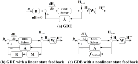
Figure 1(a) shows its system structure. Note that the current GDE methods [Jin et al., 2023] usually set uB to be equal to 0, which means it forms an uncontrolled open-loop system without external input, leading to the possibility of the system reaching an undesired over-smoothing steady state. Thus, we hope to introduce external input and state feedback to break the steady state and make the system achieve satisfactory performance. Since the system in Proposition 1 is completely observable (Please refer to Appendix A for the guarantee), meaning that the internal system state Hk can be obtained, we can establish its corresponding state feedback system.
Proposition 2. Given a control law of state feedback, i.e., u = -HkM + vL, the closed-loop feedback system corresponding to the simplified continuous graph propagation in Proposition 1 is as:
where ˆA = ˜A + I, b = vLB, B ∈ Rd×d is the control matrix, Wk ∈ Rd×d is the trainable parameter matrix, M ∈ Rd×d is the state feedback matrix, v ∈ Rn×d is the reference input, and L ∈ Rd×d is the control matrix for v.
Its system structure is shown in Figure 1(b). Note that, if B is 0, the system (3) in Proposition 2 degenerates into the linear GDE methods [Jin et al., 2023]. That is, the original simplified continuous graph propagation is a special case of the proposed feedback system. Actually, ˆAHk can be viewed as the interactions with neighbors and HkMB as the evolution of variables themselves, which is similar to the general form of network dynamics [Barzel and Barab´asi, 2013; Cui et al., 2024]. If there are external factors such as weather, i.e., the input v exists, we can learn the parameter matrix L. Otherwise, we assign L to 0 to ignore the influence of v. If not specified, we set L = 0 in our settings. Thus, we can achieve satisfactory performance by adjusting the parameter matrices (B, M, and Wk) to control the model. From the first part in Eq. 3, we see that its right-hand side consists of three parts, i.e., feature convolution (ˆAHk), linear state negative feedback (-HkMB), and a bias term. Naturally, we transform the linear state feedback part into a nonlinear one to improve the practicality, as shown in Figure 1(c).
Proposition 3. For a linear feedback system, its nonlinear extension of the continuous graph propagation can be:
where ffeedback is a nonlinear neural network.
4 SF-GDE: ProposedModel for Multivariate Time Series Forecasting
Based on the proposed graph propagation mechanism, we introduce the State Feedback enhanced Graph Differential Equations (SF-GDE) for multivariate time series forecasting.
4.1 Overview of the ProposedModel
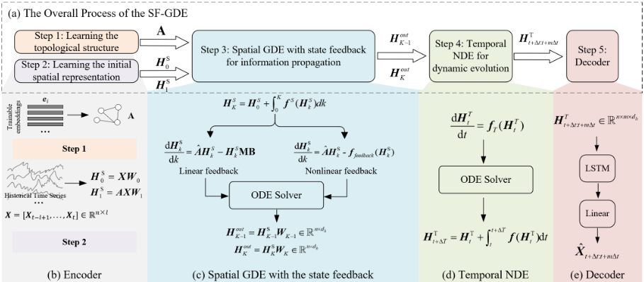
The overall process of the SF-GDE can be divided into five steps, as shown in Figure 2(a). Step 1 is to learn the spatial topological structure A that characterizes the dependency patterns between multiple time series. Step 2 is to learn the initial spatial representations from historical multiple time series to enable subsequent graph propagation, i.e., H S0 and H S1 . Then, based on the learned topological structure, Step 3 is to perform message passing for capturing spatial features and obtaining the final spatial representations, i.e., Hout K-1 and Hout K . Built on spatial representations, Step 4 is to capture temporal features and get the hidden representations at any time t, i.e., H Tt . Step 5 is to output the predictive state at any future time, i.e., ˆXt. Note that the above five steps constitute four main modules, i.e., an encoder, spatial information propagation, temporal dynamic evolution, and a decoder.
4.2 Encoder
To model the implicit topological structure for multivariate time series, we assign a learnable embedding vector, i.e., ei ∈ Rde , to each variable i, where de is the embedding dimension, and then construct the spatial topological patterns by calculating the cosine distance between variables, i.e, A, where Aij = (ei × eTj )/(∥ei∥×∥ej∥) represents the connecting weight between variables i and j, and n is the number of variables. The cosine distance is commonly used and effective for measuring the correlation between variable features. This simple way can efficiently reduce computational complexity compared to directly calculating the similarities between high-dimensional historical time series, whose length is usually much greater than de. Due to the importance of having good initial values for solving differential equations, we transform historical time series to construct initial representations (see Figure 2(b)) by H S0 = XW0,H S1 = AXW1, where, X ∈ Rn×l represents the historical multivariate time series, H S0 ∈ Rn×dh and H S1 ∈ Rn×dh are the initial representations after transformation, l is the length of historical time series, dh is the dimension of initial representations, and W0,W1 ∈ Rl×dh are learnable weights.
4.3 Spatial GDEWith the State Feedback
To overcome the over-smoothing, we build a spatial GDE based on the proposed continuous graph propagation with learnable feedback mechanism to capture spatial characteristics of multivariate time series (Figure 2(c)).
Implementation of the linear state feedback: Based on Proposition 2, ignoring the bias term, we can create the continuous graph propagation process with linear feedback as: dHSk dk = ˆAHSk -HSk MB, where HSk is the spatial representation at propagation layer k. ˆA = ˜A + I, ˜A ∈ Rn×n is the normalized adjacency matrix calculated from A, B ∈ Rdh×dh and M ∈ Rdh×dh are the trainable weights.
Implementation of the nonlinear state feedback: In the face of more complex scenarios, we propose a practical nonlinear implementation based on Proposition 3 as: dHSk dk = ˆAHSk -ffeedback(HSk ), where ffeedback is a neural network. Integral approximation of continuous graph propagation: By solving the initial value problem (IVP), we can obtain the spatial representation at any continuous layer K as: HSK = HS0 + ∫ K 0 f S (HSk )dk, where H S0 is an initial representation obtained from the encoder, f S (HSk ) = ˆAHSk - HSk MB for linear implementation and f S (HSk ) = ˆAHSk - ffeedback(HSk ) for nonlinear implementation. Due to complex neighbor interactions and nonlinearity, deriving its closed-form solution is usually intractable. Therefore, in principle, any ODE solver can be used to approximate the integral. To achieve a balance between computational efficiency and approximation accuracy, we empirically choose the Predictor-Corrector method [Abramowitz and Stegun, 1964] for numerically approximating the integral: HSk+∆k = HSk + ∆k 2 [f S (HSk ) + f S (HSk-∆k + 2∆kf S (HSk ))], where ∆k is the difference between continuous layers. Note that in this nested form, the representation of the current step, i.e., HSk+∆k , is calculated through a nonlinear transformation of the representations of the previous two steps, i.e., HSk and HSk-∆k . We thus can use the H S0 and H S1 obtained from the encoder to initiate the iterative process to obtain the spatial representation HSK . See Appendix B.1 for the detailed derivation. Then, the final spatial representation produced by the linear or nonlinear graph propagation can be calculated as Hout K = HSKWK, whereWK ∈ Rdh×dh is the weights.
4.4 Temporal NDE for Dynamic Evolution
Built on spatial representations, we introduce a temporal neural differential equation (NDE) to capture the temporal characteristics of the dynamic evolution of multivariate time series, as shown in Figure 2(d). We define the dynamic evolution process as: dH Tt dt = f T (H Tt ), where H Tt is the hidden temporal representation at time t and f T represents the learnable evolution mechanism. Given the initial temporal representation, i.e., H T0 , we can obtain the hidden temporal representation at any time t as: H Tt = H T0 + ∫ t 0 f T (H Tτ )dτ. We also use the Predictor-Corrector method [Abramowitz and Stegun, 1964] to approximate the intractable integral as: H Tt+∆t = H Tt + ∆t 2 [f T (H Tt ) + f T (H Tt-∆t + 2∆tf T (H Tt ))], where ∆t is the integration interval. Note that the temporal representation at future time t +∆t, i.e., H Tt+∆t , can be obtained by iterative calculations of the previous two steps, i.e., H Tt and H Tt-∆t . To initiate iterative computation, we set the outputs from the spatial GDE as the first two steps, i.e., H T0 = Hout K-1 and H T1 = Hout K . After m iterations, we can obtain the temporal representations in the future as H T t+∆t:t+m∆t ∈ Rn×m×dh . See Appendix B.2 for the detailed derivation.
4.5 Decoder
The decoder receives the future hidden representations H T t+∆t:t+m∆t from the temporal NDE, and then performs decoding operations to restore it to the original space of the time series as: ˆXt+∆t:t+m∆t = f De (H T t+∆t:t+m∆t ), where ˆXt+∆t:t+m∆t ∈ Rn×m is the predictions for multivariate time series and f De is a decoder, parameterized by an LSTM followed by a linear layer (see Figure 2(e)).
4.6 Loss Function
To learn the parameters in each module of SF-GDE, we design a loss function with a stability penalty as follows: L = Lpred +βLstable, where Lpred is the prediction error between predictions and ground truth, Lstable is a stability penalty, and β is a penalty coefficient. Specifically, we choose the commonly used mean square error as empirical risk, i.e., Lpred = 1 nm ∑n i=1 ∑m j=1 (Xi,j - ˆXi,j)2 , where n is the number of variables, m is the length of time series to be predicted, and Xi,j and ˆXi,j are the ground truth and prediction of variable i at step j, respectively. The most important feature of the dynamical system in the SF-GDE is its stability, as an unstable system cannot complete the expected control tasks [Erichson et al., 2019]. We, thus, add a stability penalty to the loss function to ensure the effectiveness of the SF-GDE. Here, we focus on Lyapunov's second method [Cunningham, 1962] to measure stability, which is applicable to nonlinear systems that are difficult to solve. The following two main conditions need to be considered: 1) The dynamical system has an equilibrium at the origin, i.e., f(0) = 0, where f is a differential equation. 2) We choose a quadratic scalar equation as the Lyapunov function to ensure its positive definite, i.e., V(x1:p) = x21+, . . . , +x2p , where x1:p is an p-dimensional vector, and its derivative should satisfy negative definite, i.e., ˙V < 0. Therefore, we can construct the stability penalty based on the above conditions as: Lstable = (f S (0))2 + (f T (0))2+∑k σ( ∂V(HSk ) ∂k +ξ, 0)+∑t σ( ∂V(HTt ) ∂t +ξ, 0), where f S is the differential equation in spatial GDE, f T is the differential equation in temporal NDE, σ(.) = ReLU(.), ∀k ≥ 0, ∀t ≥ 0, and ξ > 0. In implementation, we sample the k and t of intermediate states. Note that the larger ξ is, the more strictly negative definite ˙V is. The computational complexity analysis of our model can be found in Appendix C.
5 Experiment
We test the SF-GDE 1 on four real-world datasets in various fields, including air quality, climate, and transportation, to answer the following questions: 1) Can the proposed SF-GDE bring performance improvement to multivariate time series forecasting in practical applications? 2) What factors in the SF-GDE have an impact on performance? 3) Can the proposed continuous graph propagation with the state feedback mechanism boost more nonlinear GDEs?
Task description. We perform multivariate time series forecasting tasks using l historical steps to predict the next 1 to m steps, i.e., Xt-l+1:t ∈ Rn×l → ˆXt+1:t+m ∈ Rn×m. We set l and m to 5 and 10 respectively.
Datasets: Seoul PM2.5 dataset 2 contains PM2.5 concentration data collected from 25 locations from 2017 to 2019, where the data collection interval is 1 hour. PEMS04 traffic flow dataset [Song et al., 2020] contains the traffic flow of 307 locations over 59 days, with a 5-minute interval between records. Beijing temperature dataset 3 collects the temperature data from 18 regions in Beijing, China, from January 30th, 2017 to January 30th, 2018 with a sampling frequency of once an hour. A large-scale Traffic dataset [Wu et al., 2021a] contains the taffic flow of 862 locations over 61 dayse, with the same records interval as PEMS04. The division of the training, validation, and testing sets follows 6:2:2.
Baselines: We select nine representative and cutting-edge methods for comparison, which can be divided into four groups: CNN/RNN-based methods, i.e., LSTNet [Lai et al., 2018], GNN-based methods, i.e, Graph WaveNet [Wu et al., 2019b] and STGCN [Song et al., 2020], GDE-based methods, i.e., STGODE [Fang et al., 2021], TG-ODE [Gravina et al., 2024], and STDDE [Long et al., 2024], and transformerbased methods, i.e., Autoformer [Wu et al., 2021a], Crossformer [Zhang and Yan, 2023], and iTransformer [Liu et al., 2024]. SF-GDEl and SF-GDEnl are respectively denoted as linear and nonlinear implementations of our proposed mechanisms. More settings can be found in Appendix D.
1 Our source code and the accompanying appendices can be found at https://github.com/QipengW/SF-GDE.
2 www.kaggle.com/datasets/bappekim/air-pollution-in-seoul
3 https://biendata.com/competition/kdd2018
| Models | Metrics | Seoul PM2.5 Dataset | PEMS04 Dataset | Temperature Dataset | Average ranking | |||||||||
|---|---|---|---|---|---|---|---|---|---|---|---|---|---|---|
| 1 | 4 | 7 | 10 | 1 | 4 | 7 | 10 | 1 | 4 | 7 | 10 | |||
| RMSE | 2.49 | 2.90 | 3.43 | 4.13 | 34.95 | 42.98 | 50.39 | 57.10 | 1.40 | 4.16 | 6.07 | 7.26 | 8.25 | |
| LSTNet MAE | 2.18 | 2.39 | 2.49 | 2.77 | 23.12 | 28.90 | 34.29 | 39.39 | 1.00 | 3.36 | 4.96 | 5.89 | 8.25 | |
| RMSE | 0.31 | 1.03 | 2.04 | 3.09 | 25.52 | 28.63 | 43.89 | 61.33 | 4.68 | 4.89 | 6.64 | 7.27 | 5.92 | |
| GraphWaveNet MAE | 0.24 | 0.79 | 1.54 | 2.25 | 18.54 | 20.66 | 31.02 | 44.65 | 3.63 | 3.86 | 5.34 | 6.01 | 6.08 | |
| RMSE | 2.71 | 2.82 | 3.01 | 3.30 | 33.41 | 37.27 | 41.69 | 45.95 | 2.45 | 4.60 | 6.48 | 6.62 | 7.00 | |
| STGCN MAE | 2.02 | 2.14 | 2.28 | 2.56 | 21.35 | 24.26 | 27.70 | 31.18 | 1.82 | 3.46 | 4.92 | 5.15 | 6.42 | |
| RMSE | 1.34 | 1.49 | 2.26 | 3.33 | 31.48 | 37.33 | 44.14 | 51.47 | 3.66 | 5.34 | 6.92 | 7.63 | 7.67 | |
| STGODE MAE | 0.92 | 1.00 | 1.58 | 2.40 | 21.39 | 25.38 | 30.35 | 36.01 | 2.65 | 4.37 | 5.84 | 6.40 | 7.50 | |
| RMSE | 0.21 | 1.13 | 2.21 | 3.42 | 29.82 | 37.90 | 45.87 | 53.67 | 1.22 | 4.23 | 6.57 | 7.44 | 6.17 | |
| TG-ODE MAE | 0.15 | 0.82 | 1.61 | 2.51 | 18.84 | 24.86 | 30.95 | 36.97 | 0.91 | 3.59 | 5.77 | 6.33 | 6.25 | |
| RMSE | - | - | - | - | 33.34 | 35.54 | 39.49 | 43.55 | - | - | - | - | 5.25 | |
| STDDE MAE | - | - | - | - | 21.95 | 23.51 | 26.55 | 29.75 | - | - | - | - | 5.50 | |
| RMSE | 1.86 | 2.05 | 2.57 | 3.01 | 24.98 | 26.74 | 42.42 | 63.33 | 4.66 | 5.11 | 5.94 | 6.61 | 5.83 | |
| Autoformer MAE | 1.25 | 1.48 | 1.66 | 2.02 | 18.31 | 19.62 | 28.88 | 46.21 | 3.67 | 4.14 | 4.69 | 5.24 | 6.42 | |
| RMSE | 0.51 | 0.84 | 2.61 | 3.56 | 34.42 | 36.47 | 39.07 | 43.37 | 4.19 | 5.19 | 5.68 | 6.61 | 5.83 | |
| Crossformer MAE | 0.42 | 0.64 | 2.07 | 2.88 | 25.48 | 26.68 | 27.82 | 32.63 | 3.01 | 4.12 | 4.44 | 5.28 | 6.92 | |
| RMSE | 2.18 | 2.33 | 2.74 | 2.92 | 28.77 | 35.54 | 40.17 | 47.44 | 4.00 | 4.36 | 5.67 | 6.60 | 5.33 | |
| iTransformer MAE | 1.27 | 1.37 | 1.60 | 1.82 | 20.43 | 22.83 | 26.54 | 32.16 | 3.02 | 3.36 | 4.41 | 5.23 | 4.83 | |
| RMSE | 0.22 | 0.87 | 1.78 | 2.79 | 29.48 | 34.15 | 38.74 | 42.93 | 2.51 | 3.64 | 5.62 | 6.53 | 2.42 | |
| SF-GDEl MAE | 0.14 | 0.60 | 1.25 | 1.98 | 18.10 | 21.70 | 24.98 | 28.05 | 1.57 | 2.81 | 4.36 | 5.10 | 1.92 | |
| RMSE | 0.45 | 0.93 | 1.80 | 2.75 | 29.81 | 33.79 | 37.83 | 41.88 | 2.49 | 3.80 | 5.46 | 6.32 | 2.33 | |
| SF-GDEnl MAE | 0.29 | 0.64 | 1.26 | 1.93 | 18.23 | 21.43 | 24.33 | 27.33 | 1.63 | 2.92 | 4.24 | 4.93 | 2.08 | |
| Models | 1-th step 3-th step 5-th step 7-th step 10-th step | ||||
| STGCN | 0.0255 | 0.0312 | 0.0351 | 0.0382 | 0.0401 |
| TG-ODE | 0.0250 | 0.0305 | 0.0352 | 0.0359 | 0.0364 |
| Autoformer | 0.0153 | 0.0182 | 0.0279 | 0.0347 | 0.0472 |
| SF-GDEl(ours) | 0.0112 | 0.0189 | 0.0221 | 0.0233 | 0.0242 |
| SF-GDEnl(ours) | 0.0109 | 0.0185 | 0.0220 | 0.0234 | 0.0238 |
5.1 Performance Comparison
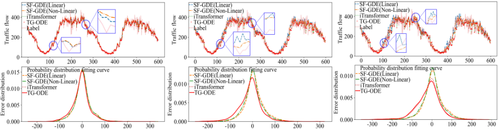
From Table 1, we see that as the future time steps that need to be predicted become longer, the model performance shows a decreasing trend, which means that medium- and long-term predictions are more difficult than short-term. The LSTNet has the worst performance mainly due to the lack of effective modeling of spatial features. By explicitly modeling spatial patterns, GNN-based and GDE-based methods have advantages in predicting multivariate time series, with an average ranking of around 5 to 7. Due to the fact that the STDDE is specifically designed for traffic flow forecasting and introduces delay estimation that requires the use of a road network, we only compared it on the PEMS04 traffic flow dataset. The transformer-based methods have good results in short-term prediction, i.e., making predictions within the next 5 steps, but perform poorly in long-term prediction, i.e., making predictions beyond the next 5 steps. In comparison, the linear implementation of state feedback, i.e., SF-GDEl, performs well in short-term prediction, while non-linear implementation, i.e., SF-GDEnl, has a significant performance improvement in long-term prediction, mainly because the real-world datasets often have strong nonlinear characteristics and nonlinear feedback can facilitate adaptive learning to more suitable representations. Overall, our SF-GDEs have the best performance, with an average ranking of around 1 to 2, far surpassing others, demonstrating that the introduction of the state feedback brings a good theoretical basis and can effectively improve performance. The comparison results on large-scale Traffic dataset also have the same observations (see Table 2). From Figure 3, we see that the predicted trends of all methods are close to the ground truth, but as the prediction steps increase, the distributions of predictive errors for the iTransformer and TG-ODE gradually show heavy tails and their means have shifted, indicating an increase in errors and the emergence of model prediction bias. Meanwhile, distributions of predictive errors from ours still form normal distributions, demonstrating that they work normally. The zoomed subplots in Figure 3 shows that, the longer the prediction step, the more local predictive bias will occur in the SF-GDEl. That is, some local trends will be opposite to the ground truth. By comparison, SF-GDEnl maintains consistency with truth, demonstrating the potential of nonlinear implementation of state feedback in practical applications, especially for long-term prediction. Additional analyses of results and baseline comparisons with consistent conclusions, including T-Mixer [Wang et al., 2024], M-TCN [Luo and Wang, 2024], and P-former [Chen et al., 2024], can be found in Appendices E.1 and E.2.
5.2 Ablation Experiment
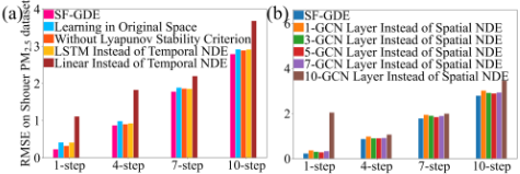
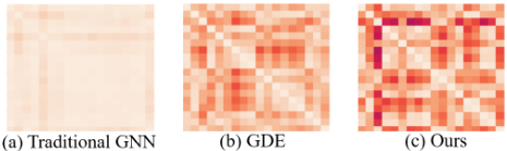
To analyze the rationality behind our SF-GDE, we conducted ablation validation on the main modules, including the initial spatial representation learning (Step 2), spatial GDE with the state feedback (Step 3), temporal NDE for dynamic evolution (Step 4), and Lyapunov stability penalty in the loss function. From Figure 4(a), we see that our SF-GDE outperforms the variants, demonstrating the effectiveness of the design of the main modules in the architecture. From Figure 4(b), our SFGDE has smaller errors compared to other shallow and deep GNN variants. Moreover, the spatial GDE with the state feedback in our SF-GDE demonstrates more discriminative representations after multiple rounds of graph propagation (see Figure 5 and Appendix E.3), effectively overcoming oversmoothing. We also validated model tolerance for noisy and missing data on a synthesized Lorentz system, and the results show that ours have stronger robustness (see Appendix E.4).
5.3 Boosting Nonlinear GDEs
The proposed feedback mechanism mainly focuses on the simplified linear GDE. Here, we propose a more general form that applies to a wider range of nonlinear GDEs to verify its applicability. For the linear feedback, we adopt the following extension: dHSk /dk = GNN(A, HSk ) - HSk MB, and for the nonlinear feedback, we use the following graph propagation: dHSk /dk = GNN(A, HSk )-f feedback (HSk ), where GNN can be any graph neural network, such as GCN and GIN. Let GDEGCN and GDEGIN respectively denote the nonlinear GDEs propagated using GCN and GIN. The methods with subscript l introduce linear feedback implementation, while those with subscript nl add nonlinear feedback implementation. Table 3 shows that methods with feedback mechanisms perform best, demonstrating that the feedback path opened up for graph propagation does indeed enhance model performance. See more results in Appendix E.5.
| Models | GCN | GDEGCN | SF-GDEGCNl | SF-GDEGCNnl |
|---|---|---|---|---|
| RMSE | 159.01(0.02) | 39.82(6.17) | 39.30(6.04) | 38.77(5.87) |
| MAE | 130.06(0.03) | 26.35(4.56) | 25.89(4.32) | 25.50(4.33) |
| Models | GIN | GDEGIN | SF-GDEGINl | SF-GDEGINnl |
| RMSE | 40.70(6.59) | 40.27(6.80) | 40.21(6.71) | 40.19(6.81) |
| MAE | 27.22(5.00) | 26.84(5.24) | 26.52(4.95) | 26.62(5.17) |
6 Conclusion
In this study, we propose a novel graph propagation to enhance the GDEs by opening up a feedback pathway for the message passing process, adaptively adjusting the representations towards the desired performance, thereby fundamentally avoiding over-smoothing. Built on the linear and non-linear implementations of the proposed propagation mechanism, we introduce the SF-GDE to effectively model multivariate time series. Comprehensive experiments on real-world datasets have demonstrated its outstanding performance. Moreover, the proposed feedback mechanism can empirically enhance any GDEs in a plug-and-play manner. Nevertheless, challenges persist in efficiently and effectively modeling multivariate relationships, higher dimensional states, and heterogeneous graphs. Further inferring the governing equations of multivariate time series, and providing support for subsequent mathematical analysis and regulation, is also crucial for explainable artificial intelligence.
Acknowledgments
This work was supported by the National Key R&D Program of China (Grant No. 2021ZD0112500), National Natural Science Foundation of China (Grant Nos. U22A2098, 62172185, 62206105 and 62202200), Natural Science Foundation of Jilin Province (Grant No. 20250102211JC), Scientific Research Project of Education Department of Jilin Province (Grant No. JJKH20250118KJ), Jilin Province Youth Science and Technology Talent Support Project (Grant No. QT202225), and Jilin Province Major Science and Technology Special Project (Grant No. 20230301002ZD).
@inproceedings{ijcai2025p820,
  title     = {State Feedback Enhanced Graph Differential Equations for Multivariate Time Series Forecasting},
  author    = {Cui, Jiaxu and Wang, Qipeng and Zhao, Yiming and Sun, Bingyi and Wang, Pengfei and Yang, Bo},
  booktitle = {Proceedings of the Thirty-Fourth International Joint Conference on
               Artificial Intelligence, {IJCAI-25}},
  publisher = {International Joint Conferences on Artificial Intelligence Organization},
  editor    = {James Kwok},
  pages     = {7374--7382},
  year      = {2025},
  month     = {8},
  note      = {Main Track},
  doi       = {10.24963/ijcai.2025/820},
  url       = {https://doi.org/10.24963/ijcai.2025/820},
}
TY - CPAPER TI - State Feedback Enhanced Graph Differential Equations for Multivariate Time Series Forecasting AU - Cui, Jiaxu AU - Wang, Qipeng AU - Zhao, Yiming AU - Sun, Bingyi AU - Wang, Pengfei AU - Yang, Bo T2 - Proceedings of the Thirty-Fourth International Joint Conference on Artificial Intelligence, IJCAI-25 PB - International Joint Conferences on Artificial Intelligence Organization PY - 2025 SP - 7374 EP - 7382 DO - 10.24963/ijcai.2025/820 UR - https://doi.org/10.24963/ijcai.2025/820 ER -Copied
Machine-readable versions of this paper, for tools and AI agents:





