
Deterministic Binary Filters for Convolutional Neural Networks
Proceedings of the Twenty-Seventh International Joint Conference on Artificial Intelligence. Main track. Pages 2739-2747.
https://doi.org/10.24963/ijcai.2018/380
Keywords
- Machine Learning: Deep Learning
- Computer Vision: Computer Vision
Abstract
We propose Deterministic Binary Filters, an approach to Convolutional Neural Networks that learns weighting coefficients of predefined orthogonal binary basis instead of the conventional approach of learning directly the convolutional filters. This approach results in model architectures with significantly fewer parameters (4x to 16x) and smaller model sizes (32x due to the use of binary rather than floating point precision). We show our deterministic filter design can be integrated into well-known network architectures (such as ResNet and SqueezeNet) with as little as 2% loss of accuracy (under datasets like CIFAR-10). Under ImageNet, they result in 3x model size reduction compared to sub-megabyte binary networks while reaching comparable accuracy levels.
- [Adachi et al., 1997] F. Adachi, M. Sawahashi, and K. Okawa. Tree-structured generation of orthogonal spreading codes with different lengths for forward link of ds-cdma mobile radio. Electronics Letters, 33(1):27-28, Jan 1997.
- [Adachi et al., 1998] Fumiyuki Adachi, Mamoru Sawahashi, and Hirohito Suda. Wideband ds-cdma for next-generation mobile communications systems. IEEE communications Magazine, 36(9):56-69, 1998.
- [Andreev et al., 2003] Boris D. Andreev, Edward L. Title- baum, and Eby G. Friedman. Orthogonal code generator for 3g wireless transceivers. In Proceedings of the 13th ACM Great Lakes Symposium on VLSI, GLSVLSI '03, pages 229-232, New York, NY, USA, 2003. ACM.
- [Bhattacharya and Lane, 2016a] S. Bhattacharya and N. D. Lane. From smart to deep: Robust activity recognition on smartwatches using deep learning. In 2016 IEEE Interna- tional Conference on Pervasive Computing and Communi- cation Workshops (PerCom Workshops), pages 1-6, March 2016.
- [Bhattacharya and Lane, 2016b] Sourav Bhattacharya and Nicholas D. Lane. Sparsification and separation of deep learning layers for constrained resource inference on wear- ables. In Proceedings of the 14th ACM Conference on Em- bedded Network Sensor Systems CD-ROM, SenSys '16, pages 176-189, New York, NY, USA, 2016. ACM.
- [Courbariaux and Bengio, 2016] Matthieu Courbariaux and Yoshua Bengio. Binarynet: Training deep neural net- works with weights and activations constrained to +1 or -1. CoRR, abs/1602.02830, 2016.
- [Esser et al., 2015] Steve K Esser, Rathinakumar Ap- puswamy, Paul Merolla, John V. Arthur, and Dharmen- dra S Modha. Backpropagation for energy-efficient neuromorphic computing. In Advances in Neural Infor- mation Processing Systems 28, pages 1117-1125.
- Curran Associates, Inc., 2015.
- [Fernandez-Marques et al., 2018] Javier Fernandez- Marques, Vincent T.-S. Tseng, Sourav Bhattacharya, and Nicholas D. Lane. On-the-fly deterministic binary filters for memory efficient keyword spotting applications on embedded devices. In Proceedings of the 2nd Inter- national Workshop on Deep Learning for Mobile Systems and Applications, EMDL '18. ACM, 2018.
- [Frosst and Hinton, 2017] Nicholas Frosst and Geoffrey E. Hinton. Distilling a neural network into a soft decision tree. CoRR, abs/1711.09784, 2017.
- [Georgiev et al., 2017] Petko Georgiev, Nicholas D. Lane, Cecilia Mascolo, and David Chu. Accelerating mobile au- dio sensing algorithms through on-chip gpu offloading. In Proceedings of the 15th Annual International Conference on Mobile Systems, Applications, and Services, MobiSys '17, pages 306-318, New York, NY, USA, 2017. ACM.
- [Han et al., 2015] Song Han, Huizi Mao, and William J. Dally. Deep compression: Compressing deep neural net- work with pruning, trained quantization and huffman cod- ing. CoRR, abs/1510.00149, 2015.
- [He et al., 2015] Kaiming He, Xiangyu Zhang, Shaoqing Ren, and Jian Sun. Deep residual learning for image recog- nition. CoRR, abs/1512.03385, 2015.
- [Howard et al., 2017] Andrew G. Howard, Menglong Zhu, Bo Chen, Dmitry Kalenichenko, Weijun Wang, Tobias Weyand, Marco Andreetto, and Hartwig Adam. Mo- bilenets: Efficient convolutional neural networks for mo- bile vision applications. CoRR, abs/1704.04861, 2017.
- [Iandola et al., 2016] Forrest N. Iandola, Matthew W. Moskewicz, Khalid Ashraf, Song Han, William J. Dally, and Kurt Keutzer. Squeezenet: Alexnet-level accuracy with 50x fewer parameters and <1mb model size. CoRR, abs/1602.07360, 2016.
- [Jarrett et al., 2009] Kevin Jarrett, Koray Kavukcuoglu, Marc'Aurelio Ranzato, and Yann LeCun. What is the best multi-stage architecture for object recognition? In IEEE 12th International Conference on Computer Vision, ICCV 2009, 2009.
- [Juefei-Xu et al., 2017] Felix Juefei-Xu, Vishnu Naresh Boddeti, and Marios Savvides. Local binary convolutional neural networks. In Computer Vision and Pattern Recogni- tion (CVPR), 2017 IEEE Conference on, volume 1, 2017.
- [Kim et al., 2009] S. Kim, M. Kim, C. Shin, J. Lee, and Y. Kim. Efficient implementation of ovsf code genera- tor for umts systems. In 2009 IEEE Pacific Rim Confer- ence on Communications, Computers and Signal Process- ing, pages 483-486, Aug 2009.
- [Krizhevsky et al., 2012] Alex Krizhevsky, Ilya Sutskever, and Geoffrey E Hinton. Imagenet classification with deep convolutional neural networks. In Advances in Neural In- formation Processing Systems 25, pages 1097-1105.
- [Lane et al., 2015] Nicholas D. Lane, Sourav Bhattacharya, Petko Georgiev, Claudio Forlivesi, and Fahim Kawsar. An early resource characterization of deep learning on wear- ables, smartphones and internet-of-things devices. In Pro- ceedings of the 2015 International Workshop on Internet of Things Towards Applications, IoT-App '15, pages 7-12, New York, NY, USA, 2015. ACM.
- [Lane et al., 2017] N. D. Lane, S. Bhattacharya, A. Mathur, P. Georgiev, C. Forlivesi, and F. Kawsar. Squeezing deep learning into mobile and embedded devices. IEEE Perva- sive Computing, 16(3):82-88, 2017.
- [LeCun et al., 1989] Y. LeCun, B. Boser, J. S. Denker, D. Henderson, R. E. Howard, W. Hubbard, and L. D. Jackel. Backpropagation applied to handwritten zip code recognition. Neural Comput., 1(4):541-551, December 1989.
- [Mathur et al., 2017] Akhil Mathur, Nicholas D. Lane, Sourav Bhattacharya, Aidan Boran, Claudio Forlivesi, and Fahim Kawsar. Deepeye: Resource efficient local execu- tion of multiple deep vision models using wearable com- modity hardware. In Proceedings of the 15th Annual In- ternational Conference on Mobile Systems, Applications, and Services, MobiSys '17, pages 68-81, New York, NY, USA, 2017. ACM.
- [McDanel et al., 2017] Bradley McDanel, Surat Teerapit- tayanon, and H. T. Kung. Embedded binarized neural net- works. In Proceedings of the 2017 International Confer- ence on Embedded Wireless Systems and Networks, EWSN 2017, Uppsala, Sweden, February 20-22, 2017, pages 168-173, 2017.
- [Pinto et al., 2009] Nicolas Pinto, David Doukhan, James J. DiCarlo, and David D. Cox. A high-throughput screen- ing approach to discovering good forms of biologically inspired visual representation. PLOS Computational Bi- ology, 5:1-12, 11 2009.
- [Purohit et al., 2013] G. Purohit, V. K. Chaubey, K. S. Raju, and P. V. Reddy. Fpga based implementation and testing of ovsf code. In 2013 International Conference on Advanced Electronic Systems (ICAES), pages 88-92, Sept 2013.
- [Rastegari et al., 2016] Mohammad Rastegari, Vicente Or- donez, Joseph Redmon, and Ali Farhadi. Xnor-net: Ima- genet classification using binary convolutional neural net- works. CoRR, abs/1603.05279, 2016.
- [Rintakoski et al., 2004] T. Rintakoski, M. Kuulusa, and J. Nurmi. Hardware unit for ovsf/walsh/hadamard code generation [3g mobile communication applications]. In 2004 International Symposium on System-on-Chip, 2004. Proceedings., pages 143-145, Nov 2004.
- [Saxe et al., 2011] Andrew Saxe, Pang W. Koh, Zhenghao Chen, Maneesh Bhand, Bipin Suresh, and Andrew Y. Ng. On random weights and unsupervised feature learning. In Proceedings of the 28th International Conference on Ma- chine Learning (ICML-11). ACM, 2011.
- [Soudry et al., 2014] Daniel Soudry, Itay Hubara, and Ron Meir. Expectation backpropagation: Parameter-free train- ing of multilayer neural networks with continuous or dis- crete weights. In Advances in Neural Information Process- ing Systems 27, pages 963-971.
- Curran Associates, Inc., 2014.
- [Suleiman et al., 2017] A. Suleiman, Y. H. Chen, J. Emer, and V. Sze. Towards closing the energy gap between hog and cnn features for embedded vision. In 2017 IEEE In- ternational Symposium on Circuits and Systems (ISCAS), pages 1-4, May 2017.
- [Sze et al., 2017] Vivienne Sze, Yu-Hsin Chen, Tien-Ju Yang, and Joel S. Emer. Efficient processing of deep neural networks: A tutorial and survey. CoRR, abs/1703.09039, 2017.
- [Tahavori et al., 2017] Fatemeh Tahavori, Emma Stack, Veena Agarwal, Malcolm Burnett, Ann Ashburn, Seyed Amir Hoseinitabatabaei, and William Harwin. Physical activity recognition of elderly people and people with parkinson's (pwp) during standard mobility tests using wearable sensors. In Smart Cities Conference (ISC2), 2017 International, pages 1-4. IEEE, 2017.
- [Vanhoucke et al., 2011] Vincent Vanhoucke, Andrew Se- nior, and Mark Z. Mao. Improving the speed of neural networks on cpus. In Deep Learning and Unsupervised Feature Learning Workshop, NIPS 2011, 2011.
- [Wang et al., 2016] Yunhe Wang, Chang Xu, Shan You, Dacheng Tao, and Chao Xu. Cnnpack: Packing convolu- tional neural networks in the frequency domain. In D. D. Lee, M. Sugiyama, U. V. Luxburg, I. Guyon, and R. Gar- nett, editors, Advances in Neural Information Processing Systems 29, pages 253-261.
- Curran Associates, Inc., 2016.
- [Yao et al., 2017] Shuochao Yao, Yiran Zhao, Aston Zhang, Lu Su, and Tarek F. Abdelzaher. Compressing deep neural network structures for sensing systems with a compressor- critic framework. CoRR, abs/1706.01215, 2017.
References were extracted automatically from the PDF and may contain errors.
Full text extracted automatically from the PDF; figures, tables and equations may differ. The PDF is the version of record.
1 Introduction
Since the success of AlexNet [Krizhevsky et al., 2012], convolutional neural networks (CNN) have become the preferred option for computer vision related tasks. While traditionally the research community has been fixated on goals such as model generalization and accuracy in detriment of model size. Recently, multiple approaches attempt to reduce model's on-device memory footprint while still maintaining high levels of accuracy. Such approaches could be subdivided into two main categories: new network compression techniques and novel layer architectural designs. Multiple network compression techniques [Wang et al., 2016; Han et al., 2015; Frosst and Hinton, 2017] have been proposed as posttraining stages. In addition, several approaches, [Courbariaux and Bengio, 2016; Rastegari et al., 2016], proved the suitability of aggressive data quantisation techniques as a way to reduce the memory and compute requirements during inference by replacing 32-bit parameters with 8-bit and/or binary values. Examples of novel layer design are [He et al., 2015; Howard et al., 2017] aiming all of them to offer alternative approaches to the traditional convolutional layers, being their advantages more noticeable when operating with very highdimensional feature maps in deeper layers of the network.
In this work, we present Deterministic Binary Filters (DBF), an approach to Convolutional Neural Networks that learns weighting coefficients of predefined orthogonal binary bases instead of the conventional approach of learning directly the convolutional filters. We generate the filters as a linear combination of orthogonal binary codes that can be generated very efficiently on real time. We achieve this by using a popular orthogonal binary code generator that has been extensively studied for over two decades in the wireless community and widely used in mobile cellular systems. Our work lies in the intersection between the previously mentinoned categories: compression techniques and novel architectural designs.
Our approach results in 4× to 16× reduction in the number of convolutional layer parameters to be learned, and more than 32× savings in model size due to the use of binary weights instead of floating point parameters. Unlike most of the network compression techniques, our method allows learning compressed models directly. We demonstrate our deterministic filter design can be integrated into well-known network architectures (such as ResNet [He et al., 2015] and SqueezeNet [Iandola et al., 2016]) with as little as 2% loss of accuracy under CIFAR-10. With fewer parameters such models are less prone to over-fitting and can be potentially trained with significantly less compute operations and memory needs. DBFs can also offer improved efficiency for inference on microprocessors and embedded devices. Experiments show the suitability of DBFs and their usage in networks with model size up to 3× smaller compared to already optimized binary networks while offering comparable accuracy levels for datasets like ImageNet, which has 1000 classes.
We believe DBFs are a first step in the development of efficient architectures relying less on large amounts of trainable parameters and more on deterministic data structures. Models with such characteristics would be more suitable for applications on resource constrained embedded devices requiring high accuracy rates but minimal compute complexity. In this work we offer the following contributions:
- A new module that performs convolution filters using a weighted combination of orthogonal binary bases that offers significantly reductions on the amount of learnable parameters required for the network.
- We find that such a module is able to offer nearly equal accuracy levels under common network architectures
- and datasets, making it a viable model choice, and providing insights into filter design moving forward.
- The ability to trade-off model size for low-complexity compute, this is a unique characteristic important for low-memory platforms.
- The number of parameters needed to be updated during training can be greatly reduced since we only need to update the weights and not the entire filter, leading to a faster training and inferences stages.
2 RelatedWork
Our study of DBFs for CNNs touch upon the following areas of deep neural network research.
Novel Filter Design. The design of filters within convolutional networks is critical to the effectiveness of such networks in discriminative tasks, and have significant downstream implications for efficiency (e.g., requirements for memory and compute). Earlier work [Jarrett et al., 2009] showed random kernels with no learning achieving decent performance in Caltech-101. Similarly, other works [Saxe et al., 2011; Pinto et al., 2009] make use of random filters to show that in addition to the convolutional filters, the network architecture plays a fundamental role in the learning process. Moreover, [Saxe et al., 2011] argued that some performance of certain state-of-the-art methods can be attributed to the their architecture alone. All of these demonstrate the ability for filters despite not being learned from data during training. More closely to our filter design is the LBCNN (Local Binary CNN) module [Juefei-Xu et al., 2017] that use pre-defined sparse local binary filters that also do not need to be updated during training. However, a critical difference in our design is our ability to generate DBFs on the fly through efficient algorithms that enable significantly smaller model sizes as light-weight compute operations replaces in-memory overhead (critical for embedded and mobile scenarios with low memory footprints). LBCNN modules also cannot directly replace conventional filters in existing architectures as requires a two stage approximation of convolution. This may not be applicable to all architectural designs. In comparison, our DBFs can be trivially applied to common architectures.
Binary Networks. Adoption of network architecture designs that include binary filters and weights are also a promising direction. Under this approach parameters are represented with only one bit, reducing the model size by 32×. Although such methods offer small model size and inference efficiency they do not necessarily reduce the amount of parameters as offered by our deterministic binary filters. Expectation BackPropagation (EBP) [Soudry et al., 2014] proposes a variational Bayes method for training deterministic Multilayer Neural Networks, using binary weights and activations. This and a similar approach [Esser et al., 2015] give great speed and energy efficiency improvements. However, the improvement is still limited as binarised parameters were only used for inference. Many other proposed binary networks suffer from the problem of not having enough representational power for complex computer vision tasks, e.g. BNN [Courbariaux and Bengio, 2016], DeepIoT [Yao et al., 2017], eBNN [McDanel et al., 2017] are unable to support the complex ImageNet dataset seen in our results.
Network Architecture Optimization. Many attempts towards optimizing network architectures for more efficient training, inference and parameter exist. One direction in quantization involves taking a pre-trained model and normalizing its weights to a certain range. This is done in [Vanhoucke et al., 2011] which uses an 8 bits quantization to store activations and weights. Other works such as [Han et al., 2015] and [Wang et al., 2016] are a conglomerate of multiple clustering, quantisation and word encoding techniques that have been proven to work well in large architectures such as AlexNet and ResNet. In addition to compressing weights in neural networks, researchers have also been exploring more light-weight architectures: SqueezeNet uses 1 × 1 filters in combination with 3 × 3 filters, reducing the model to 50× smaller than AlexNet while maintaining the same accuracy levels; bottleneck layers, introduced in ResNet, that aims to reduce the number operations and parameters of convolutional layers by reducing the number of channels of the input tensor using 1×1 filters; or MobileNets [Howard et al., 2017] that make use of depthwise convolutional layers and result in lightweight networks suitable for embedded vision applications. SparseSep [Bhattacharya and Lane, 2016b] adds sparsification to both convolutional and dense layers resulting in highly compact model representations.
Deep Learning for embedded platforms. Energy efficiency and low computational complexity are two major requirements that algorithms must fulfil when deploying them in memory and compute restricted platforms [Lane et al., 2015] and they become a major concern when considering the commercialization of such applications. Embedded deep learning applications, often instantiated as wearables, exist for a diverse range applications including vision [Mathur et al., 2017; Suleiman et al., 2017], audio [Fernandez-Marques et al., 2018; Georgiev et al., 2017] and activity recognition [Tahavori et al., 2017; Bhattacharya and Lane, 2016a]. We refer the interested reader to [Lane et al., 2017] and [Sze et al., 2017] for a deeper evaluation of the challenges associated with this area of research.
3 Deterministic Binary Filters
In this section, we introduce a novel approach of performing convolution operations and present an efficient algorithm for training the parameters. Specifically, we design a convolution layer, where all filter kernels are generated using a linear superposition of a predefined bases set of binary orthogonal vectors. Fewer number of tunable parameters generates a model with a smaller memory footprint, which is particularly suitable for deployment on resource-constrained wearable or IoT devices. The properties of the binary codes used to generate the filters also makes it possible to implement convolu- Binary basis vectors
-1.0
-8.3
-0.2
-1.9
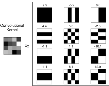
Figure 1: Overview of representing a convolution kernel using a set of binary mutually orthogonal basis vectors. The convolutional kernel (on the left) can be represent accurately using linear superposition of all the binary vectors (patches) presented on the right. The coefficient or strength of a binary vector used in the reconstruction is given on top of the patches.
tions without explicitly having the filters allocated in RAM, therefore allowing efficient runtime on embedded devices.
In this work we employ orthogonal variable spreading factor (OVSF) codes to generate filters for the convolution layer. The presented technique can also be applied to the fully connected layer parameters, however, we only focus on convolution layers in this work. In the following three sub-sections we present the main intuition behind representing convolution kernels with OVSF codes, present technique to efficiently use the codes to generate kernels and lastly describe the featuremaps generation process.
3.1 OVSF Codes: Overview
A point x ∈ RN can be represented by the span of a set of N mutually orthogonal set of vectors or bases {Bi}Ni=1 (Bi ∈ RN ), where ∀i, j, and i ̸= j, Bi ⊥ Bj. In other words, any point in RN can be presented as a linear combination of the basis vectors as:
(1)
where, αi is the coefficient or strength for the ith basis vector.
Without a loss of generality, we can apply the same linear superposition strategy when generating the hypermatrix or tensor that would become our convolutional filter. To gain computational or representational benefits, we can enforce certain properties on the bases set. For instance, in this work we only consider binary basis vectors, i.e., Bi ∈ {-1, +1}N , ∀i. For illustration, in Figure 1 we present a scenario when a random filter of dimension 4 × 4 is represented accurately by a set of 16 binary and mutually orthogonal basis vectors. The coefficients for individual binary vectors are presented on the top of each patches. Note that, for illustration purpose we only consider 2D filters, whereas in practice the filters used in convolution layers are 3D.
To achieve this filter representation, we require a techniques for efficiently generating the basis vector set. Specifically, given the dimensionality of a filter, the bases generation technique should output all the orthogonal binary vectors for the convolution parameter space. This bases generator should have the following properties: (i) capable of generating all the bases for any space regardless of its dimensionality, (ii) employs a deterministic procedure, i.e., for a given dimension, the basis vectors set remains invariant, (iii) being efficient such that it can be used in real-time applications on embedded devices.
OVSF Codes
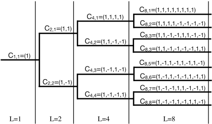
For the purpose of generating convolutional kernels, while meeting the above mentioned conditions, we use the algorithm presented in [Adachi et al., 1998]. The OVSF codes have been extensively studied in the wireless community [Andreev et al., 2003; Rintakoski et al., 2004; Kim et al., 2009; Purohit et al., 2013] and widely used in W-CDMA based 3G 1 mobile cellular systems to provide multi-user network access. Their simplicity and efficiency on-silicon implementation makes them suitable for real-time implementation on powerconstrained devices. OVSF codes are binary {-1,+1}, orthogonal to each other and of length L = 2l , l ∈ N. Figure 2 shows OVSF bases at different l values generated as a recursive process in a binary tree [Adachi et al., 1997].
3.2 Filter Generation Process
Unlike in standard CNNs, our architecture does not learn convolutional filters directly. Instead, it learns the coefficient for the basis vectors needed to generate the convolutional filters. Note that the dimension of the OVSF code is the same as the N filters, which is W ×H×C, where W and H are the width and height of the filters 2 , and C is the number of channels.
For any given code length L, there are L different OVSF codes (as observable in Figure 2). Therefore, to generate a filter of dimensions dim = W ×H ×C, our generator could output at most dim different codes that would form a basis of Rdim. Intuitively, by combining all OVSF codes of bi = [b 1
1 3GPP TS 25.213, v 3.0.0, Spreading and modulation (FDD), Oct. 1999
2 In this work we only consider square filters with dimension of the form 2l .
i , b 2
b N
b N
i = [0, 1, 1, 0, ...1]
i , b 3

i , ... ˜b N
i = [1,-1, 2, 1, ... -1]
{[1 1 1 1 ] , [ 1 1 -1 -1 ]} basisOVSF = {[1, 1, 1, 1], [1, 1, -1, -1]} Reshape + [-0.2 -0.2 1.2 1.2 ] OVSF codes Weights {0.5, -0.7} Convolutional Filter a given dimension dim we could perfectly represent any filter of that dimension. On the other hand, using fewer OVSF codes would result in a coarser representation of the target filter. Mathematically, the quality of a filter generated by combination of OVSF codes could be measured as:
where ρ ∈ [0, 1] is the ratio of codes to use in order to approximate filter fk, l is the total number of OVSF codes of length l = WHC, Bik is the ith OVSF code and αij ∈ R its associated weight. ϵ is the difference between the the approximated DBF, f ′k , and the real filter, fk. Intuitively, ϵ → 0 as we increase the ratio of binary codes used. When ρ ̸= 1, the product p · l is rounded to the nearest integer value.
Filter Generation Stages
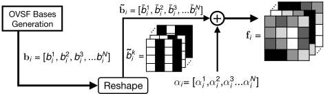
During training, the set of weights {α}Ni=1 that pre-multiply each of the OVSF codes are learnt via backpropagation [LeCun et al., 1989]. At inference time, the generated filter f ′k can be treated as any other standard floating-valued convolutional filter. The filter generation process using OVSF bases and the learned weights is didactically illustrated in Figure 3. This process involves: generation of ⌊ρ · l⌋ OVSF codes of length l = W ×H ×C; reshape each code in order to match the shape of the filter; and combine them using the learnt weights {α}Ni=1 .
The Importance of Ratios
One of the main focus of our evaluation is the study of how ρ impacts on the performance of our models. This parameter, that can be independently set for each convolutional layer in the network, is directly proportional to the number of learnable parameters N in a given layer. As an example, when ρ = 0.5, the filter would be generated using half of the OVSF codes and, therefore, our network would only require to learn half to the weights.
OVSF Limitations
By design, OVSF codes must be of length L = 2l , l ∈ N. This means that commonly used filter dimensions such as 3× 3 or 5 × 5 are not a possibility. We overcome this limitation by only using a portion of the elements in each OVSF code. For example, in order to construct a 3 × 3 × 1 × 1 filter, we i ] wi = [w 1 i ,w 2 i ,w 3 i , ...w N i ] b k i = [1,-1, 2, 1, ... - 2] would first generate OVSF codes of length 4×4×1×1; then keep 9 out of the 16 dimensions; and proceed with the reshape and combination stages as shown in Figure 3. This approach results in pseudo-OVSF codes that are no longer orthogonal to each other. We call these codes square-pseudo OVSF, spOVSF for brevity. In Section 4, we empirically show that the generated filters perform well even though the codes used are no longer mutually orthogonal.
Algorithm 1 Training with DBFs
Input: A minibatch of inputs labels and labels(X, Y ), a dictionary of orthogonal binary bases {B1,B2, ...,Bk} for each convolution filter and learning rate η.
Output: Updated coefficients {αt+1 1 , αt+1 2 , ..., αt+1 k } for each of the binary filters.
for l = 1 to L do
1. Forward Propagation:
{B1,B2, . . . ,Bk}←OVSF(n, k)
f t ← αt1B1 + αt2B2 + . . . + αtkBk
Compute X ∗ f t ▷ ∗ is the convolution operation.
2. Backward Propagation:
for i=1 to k, do
3. Coefficient Update:
for i=1 to k
3.3 Model Training and Optimization
In the following we describe the main steps involved in the training of the proposed architecture. We use stochastic gradient descent (SDG) to update all the tunable parameters in the architecture and an overview of the training process is presented in Algorithm 1. During the forward pass, we first generate individual filters, and then follow the conventional CNN inferencing to compute the loss. However, during the backward pass, we only update the coefficients {α}Ni=1 , but not the binary basis vectors. The loss propagates to each of the layers from the output layer, and the gradient of each coefficient with respect to the the total loss is calculated using chain rule, i.e.:
where L is the loss, fj is the convolution filter. During the forward propagation in the next iteration, the filters is generated using the updated coefficients.
Convolution kernel generation using OVSF codes as binary basis vectors can be easily integrated to existing architectures, such as fully CNNs, ResNet or any architecture employing convolutions. Therefore, existing architectures can be trained faster, as we have smaller number of free parameters to update, and can have better inference time.
3.4 Inference
The convolution operations within a layer, using the set of OVSF codes, can be summarized as:
where, F I is the input feature-map and F O k is the output feature-map for filter k, Bik and αik are the binary vector and corresponding coefficient while representing the kth filter. Interestingly, we can use the linearity of the convolution operation and compute the same output feature-map as follows:
These two formulations allow two distinct architecture deployment methods that are suitable in two different application scenarios. In the first case, we generate a static version of the model, employing Equation 4, and in the latter case, for resource constrained devices, we instantiate a dynamic version of the architecture where the OVSF codes are generated on the fly and then used during convolution convolutions as in Equation 5. In the following we describe the two cases.
Explicit FilterGeneration. In scenarios with sufficient ondevice memory to store the model in memory, the DBFs could be generated, and therefore allocated in memory, as part of a initialization stage during model deployment and set-up. After this, the inference stage would be identical to that of any other CNN architecture.
On-the-fly convolutions. Due to the nature of the filter generation process by combining OVSF codes using weighting coefficients learned during training we could bypass the generation and allocation of the filters during model deployment. These filters would no longer need to be explicitly generated. Instead, since our model has the weighting coefficient and we can generate OVSF codes very efficiently, we can subdivide the operations of a convolutional layer into smaller operations that are less memory taxing. Effectively, this strategy trades memory for computations.
4 Evaluation
In this section we validate the usage of DBFs in convolutional networks for the task of image classification. Here we:
- Compare the performance of two popular CNNs architectures when using filters generated from OVSF codes against standard fully-learnable filters.
- Make use of DBFs a as model size reduction strategy.
- Validate the usage of sp-OVSF codes that would permit the usage of filter with arbitrary dimensionality.
4.1 Datasets
We conducted our experiments on three popular datasets, ImageNet, CIFAR-10 and MNIST. ImageNet is a large-scale image classification dataset, which contains 1000 categories and a total of 1.33 million color images. These images vary in dimension and resolution and are generally resized and cropped to 224×224 images. The dataset is divided into training and validation data, with 1.28 million images and 50,000 images, respectively. The CIFAR-10 dataset contains 60,000 32×32 color images in 10 classes, with 6,000 images per class. There are 50,000 training images and 10,000 test images, with equal number of images per class in both training set and test set. The MNIST dataset consists of 28×28 grayscale images of handwritten digits, with 60,000 training images and 10,000 test images.
4.2 Experimental Setup
Filters generated using OVSF codes can be used in any CNN for both training and inference. In order to validate the representation capabilities of these filters, we substitute the standard convolutional layers of two popular CNN architectures, ResNet and SqueezeNet, and train them on CIFAR-10 for 250 epochs. We used batch size of 128, initial learning rate of 0.1 with decay factor of 0.1 at epochs {90, 150, 190, 220}. We applied standard dat augmentation: random image cropping, random mirroing and image normalization. We evaluate our architecture on two configuration of ResNet with 18 and 34 layers. The architectures evaluated in this section were originally designed for ImageNet, here, they have been adapted to the dimensionality of the CIFAR-10 dataset. This adaptation consist on reducing the filter dimensions and stride of the input convolutional layer.
Quality of OVSF filters. Given that OVSF codes are limited to be of length 2l , l ∈ N, we have modified the spatial dimensions (width and height) of all the 3×3 and 7×7 the convolutional filters in ResNet and SqueezeNet, and replace them with 4×4 and 8×8 filters, respectively. In Table 1 (right) we compare the accuracy levels reached for each architecture when learning filters directly and when using the proposed OVSF filter generation stage.
sp-OVSF: Overcoming 2l limitation. Despite not being the focus of this work, we evaluated the suitability of OVSF codes to generate filters whose dimensions are not a 2l , e.g. those with spatial dimensions 3×3 or 5×5. To achieve this, each time we require an OVSF code of l′ , we first generate the shortest OVSF code of dimensionality 2l > l′ , and then clip it. The resulting set of sp-OVSF codes are no longer orthogonal to each other, limiting the performance of the generated filters. In Table 1 (left) we should that these codes can still be use to generate convolutional filters.
The impact of ratios. The nature of the filter generation process using OVSF codes permits, by means of a hyperparameter, choose how many bases use to generate each convolutional filter. This hyperparamter is represented in Eq. 2
Output
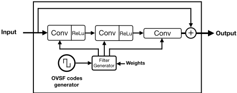
Figure 4: A three layers DBF Module.
as ρ. Lower ρ values results in fewer trainable parameters and a more efficient inference stage at the cost of generating coarser filters and a potential drop in accuracy. We evaluated the effect of using coarser filters on ResNet-18, ResNet-34 and SqueezeNet. These results are shown in Table 2. Reducing ρ effectively reduces the number of weights, α in Eq.2, needed to generate the filter and therefore resulting in a smaller model, as shown in Table 3. An architecture with DBF and ρ = 1 has the same model size as it would have with standard filters.
A newCNN architecture. We designed a new CNN architecture using DBFs. We will refer to it as DBFNet. Macroarchitecturally, it borrows from SqueezeNet in the sense that after an initial convolution and max-pooling layer, the remaining of the pipeline is comprised of a three cascades of convolutional modules separated by max-pooling layers. We call these blocks DBF Modules and consist of three stacked OVSF convolutional layers with a bypass connection. Our network is comprised of eight DBF Moudles arranged similarly to SqueezeNet's FireModules. Figure 4 shows a generic DBF Module in isolation with explicit filter generation. When part of a network, a single OVSF code generator is enough to generate the convolutional filters of the entire network. This architecture is evaluated on MNIST, CIFAR-10 and ImageNet at different ρ values. The results are shown in Table 4. On ImageNet we used learning rate of 0.1 and decay factor of 0.1 every 30 epochs for a total of 100 epochs using bach size 64. For CIFAR-10 and MNIST datasets we used batch size of 128, the same initial learning rate and decay factor but decaying it at epochs {40, 70, 90}. No pre-processing or data augmentation was applied.
4.3 Results
We have proven that, despite the simplicity of the filter generation process using binary OVSF codes, CNNs can perform as well as if filters were learnt directly, like most CNNs do. As we described in Eq.2, the proposed DBFs are as good as any other standard convolutional filter. This is shown in Table 1 (left). We have validated this on two popular deep convolutional architectures, ResNet and SqueezeNet.
Using Coarser DBFs
Networks using DBFs in their convolutional layers can adjust their memory footprint by tuning ρ. This parameter can be set independently for each convolutional layer and is used to determine the number of OVSF codes a generator should output in order to generate a given convolutional filter. We demonstrate that even a 4× reduction in the number of parameters of popular architectures such as ResNet and SqueezeNet can result in only 2% accuracy loss. In our experiments we found that reducing ρ for deeper convolutional layer has a lesser impact on accuracy than in the first layers of the network. Concretely, ρ was set to 6.25% for the last two layers in ResNet34DBF in the set up where, on average, ρ = 0.25. On the other hand, shallower layers kept ρ = 1.
| Architecture | Acc. (%) |
| ResNet-18 | 91.15 |
| ResNet-18DBF | 91.02 |
| ResNet-34 | 92.46 |
| ResNet-34DBF | 92.32 |
| SqueezeNet | 91.16 |
| SqueezeNetDBF | 91.33 |
| Architecture | Acc. (%) |
| ResNet-18 | 90.68 |
| ResNet-18sp-OVSF | 89.12 |
| ResNet-34 | 92.53 |
| ResNet-34sp-OVSF | 91.30 |
| SqueezeNet | 91.22 |
| SqueezeNetsp-OVSF | 90.25 |
| Architecture | 100% | 75% | 50% | 35% | 25% |
|---|---|---|---|---|---|
| ResNet-18DBF | 91.02 | 90.46 | 89.34 | 89.11 | 88.02 |
| ResNet-34DBF | 92.32 | 92.92 | 91.43 | 91.31 | 89.88 |
| SqueezeNetDBF | 91.33 | 91.28 | 91.17 | 89.89 | 89.22 |
| Architecture | 100% | 75% | 50% | 35% | 25% |
|---|---|---|---|---|---|
| ResNet-18DBF | 1.37 | 1.02 | 0.69 | 0.48 | 0.34 |
| ResNet-34DBF | 3.39 | 2.54 | 1.70 | 1.19 | 0.85 |
| SqueezeNetDBF | 4.41 | 3.31 | 2.21 | 1.54 | 1.10 |
To our advantage, ρ and the number of learnable parameters are tightly correlated for any architecture using DBFs. This is evidenced in Table 3. Convolutional filters of deeper layers tend to be considerably larger than those in shallower layers, as is the case in ResNet and SqueezeNet. Consequently, these filters represent a seizable portion of the total model size. By means of the parameter ρ their impact in model size can be lessened and, as previously exemplified for the case of ResNet-34DBF, it is possible to achieve 16×memory impact reduction of certain layers while maintaining good accuracy results.
Finally, we show that the benefits of using an architecture with OVSF-based filters are also applicable when the image classification task is considerable more challenging, as is the case with in the ImageNet dataset. Table 4 shows the performance of DBFNet on various image classification dataset at different ρ values.
| Dataset | 100% | 70% | 50% | 25% |
| MNIST | 99.6 | 99.6 | 99.6 | 99.5 |
| CIFAR-10 | 89.7 | 88.3 | 88.0 | 85.5 |
| ImageNet | 55.1/78.5 | 53.3/77.3 | 50.4/74.8 | 40.5/65.7 |
| Size (MB) | 10.32 | 7.25 | 5.16 | 2.58 |
5 Benefits of Deterministic Binary Filters
In the following section we present the main benefits of using the binary basis vectors for the construction of convolution filters and its effect during inference and training time.
5.1 Fewer Parameters
Results from Section 4 show that networks using DBFs offer significant parameter savings. Table 2 shows that 4× reduction in the number of total learnable parameters is possible. By means of parameter ρ we can adjust the memory impact of each layer individually, resulting in 16× memory savings in the deeper layers of the networks while maintaining their dimensionality. We believe these results can be improved by forcing the set of coefficients that pre-multiply each OVSF bases to be sparse in a layer by layer.
We demonstrated the feasibility of DBFs to reduce the model size of already small architectures, in the order of 1-4 MB in size. Our technique brings model size to levels achievable by binary networks. In Table 5 we compare ResNet18 using DBFs to two popular binary networks. BinaryConnect's results use deterministic binarization. Our technique is capable of providing similar levels of accuracy while reducing the model size to sub-MB levels. Similarly, we compare in Table 6 BinaryConnect and BWN [Rastegari et al., 2016] against our DBFNet when evaluated on ImageNet. DBFNet performs better than BinaryConnect while being 3× smaller.
| Architecture | Accuracy (%) | Size (MB) |
|---|---|---|
| BinaryConnect | 90.1 | 0.73 |
| BNN | 89.85 | 0.73 |
| ResNet-18DBF (ρ = 0.35) | 89.11 | 0.48 |
| Architecture | Top-1 (%) | Top-5 (%) | Size (MB) |
|---|---|---|---|
| BinaryConnect | 35.4 | 61.0 | 7.8 |
| DBFNet (ρ = 0.125) | 36.5 | 61.9 | 2.2 |
| BWN | 56.8 | 79.4 | 7.8 |
| DBFNet (ρ = 0.7) | 53.3 | 77.3 | 7.3 |
5.2 Inference Efficiency
During inference, the overhead of using binary bases is marginal. Bases can be generated once and used across all convolutional layers. This does not impose a big memory footprint as bases are binary and they can be densely packed into bytes and occupy 8× less space.
When these bases are expanded and combined to form the full-precision kernel we do not need to store any of the intermediate values and the run-time memory required is the same as any normal convolutional layer. However, since convolution operation is distributive and associative with scalar multiplication one can change the order of operations and do convolution of input with binary bases first and then scale and combine the results. While this approach normally does not make sense given the significant cost of convolution operation, it can be efficient in architectures with binary inputs where the convolution operation is reduced to XORing and bit counting [Rastegari et al., 2016].
5.3 Training Efficiency
The main benefits of using Deterministic Binary Filters come from their ability to reduce memory and computation footprints without a significant drop in the recognition accuracy. From the previous section we see that across different datasets the proposed architecture can achieve high accuracy while only considering a fraction of the OVSF codes. This allows for a significant reduction int the number of tunable convolution parameters, in our case only the coefficients, and generates a very compact model size, which is ideal for embedded deployment. As we need a smaller number of parameters to tune, the model becomes less prone to overfitting than the corresponding static version of the architecture. An architecture with DBFs runs faster backward pass, thereby reducing the overall training procedure significantly.
6 Conclusion
We have presented Deterministic Binary Filters, an new approach to constructing modules within CNNs that only requires learning of weighting coefficients with respect to a predefined orthogonal binary basis. Significant savings result in comparison to conventional convolutional filters that are learned entirely from data. With fewer parameters such models are less prone to over-fitting and can be potentially trained with significantly less compute operations and memory needs. DBFs provides important new insights in the design of low-complexity models that maintain high accuracy level for discriminative image tasks with implications for training and inference efficiency.
Acknowledgements
This work was supported in part by the UK's Engineering and Physical Sciences Research Council (EPSRC) with grants EP/M50659X/1, EP/N509711/1 and EP/R512333/1.
@inproceedings{ijcai2018p380,
  title     = {Deterministic Binary Filters for Convolutional Neural Networks},
  author    = {Tseng, Vincent W.-S. and Bhattacharya, Sourav and Marqués, Javier Fernández and Alizadeh, Milad and Tong, Catherine and Lane, Nicholas D.},
  booktitle = {Proceedings of the Twenty-Seventh International Joint Conference on
               Artificial Intelligence, {IJCAI-18}},
  publisher = {International Joint Conferences on Artificial Intelligence Organization},
  editor    = {Jérôme Lang},
  pages     = {2739--2747},
  year      = {2018},
  month     = {7},
  note      = {Main track},
  doi       = {10.24963/ijcai.2018/380},
  url       = {https://doi.org/10.24963/ijcai.2018/380},
}
TY - CPAPER TI - Deterministic Binary Filters for Convolutional Neural Networks AU - Tseng, Vincent W.-S. AU - Bhattacharya, Sourav AU - Marqués, Javier Fernández AU - Alizadeh, Milad AU - Tong, Catherine AU - Lane, Nicholas D. T2 - Proceedings of the Twenty-Seventh International Joint Conference on Artificial Intelligence, IJCAI-18 PB - International Joint Conferences on Artificial Intelligence Organization PY - 2018 SP - 2739 EP - 2747 DO - 10.24963/ijcai.2018/380 UR - https://doi.org/10.24963/ijcai.2018/380 ER -Copied
Machine-readable versions of this paper, for tools and AI agents:





