
Large-scale Subspace Clustering by Fast Regression Coding
Proceedings of the Twenty-Sixth International Joint Conference on Artificial Intelligence. Main track. Pages 2138-2144.
https://doi.org/10.24963/ijcai.2017/297
Keywords
- Robotics and Vision: Vision and Perception
- Machine Learning: Machine Learning
Abstract
Large-Scale Subspace Clustering (LSSC) is an interesting and important problem in big data era. However, most existing methods (i.e., sparse or low-rank subspace clustering) cannot be directly used for solving LSSC because they suffer from the high time complexity-quadratic or cubic in n (the number of data points). To overcome this limitation, we propose a Fast Regression Coding (FRC) to optimize regression codes, and simultaneously train a non-linear function to approximate the codes. By using FRC, we develop an efficient Regression Coding Clustering (RCC) framework to solve the LSSC problem. It consists of sampling, FRC and clustering. RCC randomly samples a small number of data points, quickly calculates the codes of all data points by using the non-linear function learned from FRC, and employs a large-scale spectral clustering method to cluster the codes. Besides, we provide a theorem guarantee that the non-linear function has a first-order approximation ability and a group effect. The theorem manifests that the codes are easily used to construct a dividable similarity graph. Compared with the state-of-the-art LSSC methods, our model achieves better clustering results in large-scale datasets.
- [Bengio et al., 2013] Yoshua Bengio, Aaron Courville, and Pascal Vincent. Representation learning: A review and new perspectives. IEEE Trans. Pattern Anal. Mach. Intell., 35(8):1798-1828, Aug. 2013.
- [Cai and Chen, 2015] Deng Cai and Xinlei Chen. Large scale spec- tral clustering via landmark-based sparse representation. IEEE Trans. on Cybernetics, 45(8):1669-1680, 2015.
- [Cai, 2011] Deng Cai. Litekmeans: the fastest mat- lab implementation of kmeans. In Available at: http://www.zjucadcg.cn/dengcai/Data/Clustering.html, 2011. Link
- [Chen and Cai, 2011] Xinlei Chen and Deng Cai. Large scale spec- tral clustering with landmark-based representation. In Proc. of the AAAI Conf. on Artif. Intell., pages 313-318, 2011.
- [Chen et al., 2011] Wen-Yen Chen, Yangqiu Song, Hongjie Bai, Chih-Jen Lin, and Edward Y. Chang. Parallel spectral clustering in distributed systems. IEEE Trans. Pattern Anal. Mach. Intell., 33(3):568-586, 2011.
- [Elhamifar and Vidal, 2013] Ehsan Elhamifar and Rene Vidal. S- parse subspace clustering: Algorithm, theory, and applications. IEEE Trans. Pattern Anal. Mach. Intell., 35:2765-2781, 2013.
- [Fowlkes et al., 2004] Charless Fowlkes, Serge Belongie, Fan Chung, and Jitendra Malik. Spectral grouping using the nystrom method. IEEE Trans. Pattern Anal. Mach. Intell., 26(2):214-225, 2004.
- [Gregor and LeCun, 2010] Karol Gregor and Yann LeCun. Learning fast approximations of sparse coding. In Proc. of Int. Conf. Mach. Learn., pages 399-406, 2010.
- [Haykin, 2009] Simon Haykin. In Neural Networks and Learning Machines. Pearson Education Inc., 2009.
- [Hoerl and Kennard, 2000] Arthur E. Hoerl and Robert W. Kennard. Ridge regression: Biased estimation for nonorthogonal problems. Technometrics, 42(1):80-86, 2000.
- [Kavukcuoglu et al., 2008] K. Kavukcuoglu, M. Ranzato, and Y. Le- Cun. Fast inference in sparse coding algorithms with applications to object recognition. In CBLL-TR-2008-12-01, 2008.
- [Lee et al., 2015] Minsik Lee, Jieun Lee, Hyeogjin Lee, and Nojun Kwak. Membership representation for detecting block-diagonal structure in low-rank or sparse subspace clustering. In Proc. of IEEE Conf. Comput. Vis. Pattern Recognit., pages 1648-1656, 2015.
- [Li and Vidal, 2015] Chun-Guang Li and Rene Vidal. Structured sparse subspace clustering: A unified optimization framework. In Proc. of IEEE Conf. Comput. Vis. Pattern Recognit., pages 277-286, 2015.
- [Li et al., 2015] Jun Li, Heyou Chang, and Jian Yang. Sparse deep stacking network for image classification. In Proc. of the AAAI Conf. on Artif. Intell., pages 3804-3810, 2015.
- [Li et al., 2016] Jun Li, Yu Kong, Handong Zhao, Jian Yang, and Yun Fu. Learning fast low-rank projection for image classification. IEEE Trans. Image Process., 25(10):4803-4814, 2016.
- [Li et al., 2017a] Jun Li, Yu Kong, and Yun Fu. Sparse subspace clustering by learning approximation ℓ0 codes. In Proc. of the AAAI Conf. on Artif. Intell., pages 2189-2195, 2017.
- [Li et al., 2017b] Jun Li, Tong Zhang, Wei Luo, Jian Yang, Xiaotong Yuan, and Jian Zhang. Sparseness analysis in the pertraining of deep neural networks. IEEE Trans. Neural Netw. Learn. Syst., 28(6):1425-1438, 2017.
- [Liu et al., 2007] Ting Liu, Charles Rosenberg, and Henry A. Row- ley. Clustering billions of images with large scale nearest neighbor search. In Proc. of IEEE Workshop on App. of Comput. Vis., 2007.
- [Liu et al., 2013] Guangcan Liu, Zhouchen Lin, Shuicheng Yan, Ju Sun, Yong Yu, and Yi Ma. Robust recovery of subspace struc- tures by low-rank representation. IEEE Trans. Pattern Anal. Mach. Intell., 35:171-184, 2013.
- [Lu et al., 2012] Can-Yi Lu, Hai Min, Zhong-Qiu Zhao, Lin Zhu, De-Shuang Huang, and Shuicheng Yan. Robust and efficient subspace segmentation via least squares regression. In Proc. of Euro. Conf. Comput. Vis., pages 347-360, 2012.
- [Nie et al., 2011] Feiping Nie, Zinan Zeng, Ivor W. Tsang, Dong Xu, and Changshui Zhang. Spectral embedded clustering: A framework for in-sample and out-of-sample spectral clustering. IEEE Trans. on Neural Netw., 22(11):1796-1808, 2011.
- [Peng et al., 2016] Xi Peng, Huajin Tang, Lei Zhang, Yi Zhang, and Shijie Xiao. A unified framework for representation-based subspace clustering of out-of-sample and large-scale data. IEEE Trans. Neural Netw. Learn. Syst., 27(12):2499-2512, 2016.
- [Shi and Malik, 2000] Jianbo Shi and Jitendra Malik. Normalized cuts and image segmentation. IEEE Trans. Pattern Anal. Mach. Intell., 22(8):888-905, 2000.
- [Talwalkar et al., 2013] Ameet Talwalkar, Lester Mackey, Yadong Mu, Shih-Fu Chang, and Michael I. Jordan. Distributed low-rank subspace segmentation. In Proc. of IEEE Int. Conf. Comput. Vis., pages 3543-3550, 2013.
- [Vidal, 2011] Rene Vidal. Subspace clustering. IEEE Signal Pro- cessing Magazine, 28(3):52-68, 2011.
- [Vincent et al., 2010] Pascal Vincent, Hugo Larochelle, Isabelle La- joie, Yoshua Bengio, and Pierre-Antoine Manzagol. Stacked denoising autoencoders: Learning useful representations in a deep network with a local denoising criterion. J. Mach. Learn. Res., 11:3371-3408, 2010.
- [Wang et al., 2014] Shusen Wang, Bojun Tu, Congfu Xu, and Zhi- hua Zhang. Exact subspace clustering in linear time. In Proc. of the AAAI Conf. on Artif. Intell., pages 2113-2120, 2014.
- [Xiao et al., 2014] Shijie Xiao, Mingkui Tan, and Dong Xu. Weight- ed block-sparse low rank representation for face clustering in videos. In Proc. of Euro. Conf. Comput. Vis., pages 123-138, 2014.
- [Yan et al., 2009] Donghui Yan, Ling Huang, and Michael I. Jordan. fast approximate spectral clustering. In Proc. of ACM SIGKDD Int. Conf. Knowl. Dis. and Data Min., pages 907-916, 2009.
- [Yin et al., 2016] Ming Yin, Junbin Gao, and Zhouchen Lin. Lapla- cian regularized low-rank representation and its applications. IEEE Trans. Pattern Anal. Mach. Intell., 38(3):504-517, 2016.
- [Zhang et al., 2015] Changqing Zhang, Huazhu Fu, Si Liu, Guang- can Liu, and Xiaochun Cao. Low-rank tensor constrained mul- tiview subspace clustering. In Proc. of IEEE Int. Conf. Comput. Vis., pages 1582-1590, 2015.
- [Zhao and Fu, 2015a] Handong Zhao and Yun Fu. Dual-regularized multi-view outlier detection. In Proc. of of Int. Joint Conf. on Artif. Intell., pages 4077-4083, 2015. IJCAI
- [Zhao and Fu, 2015b] Handong Zhao and Yun Fu. Semantic single video segmentation with robust graph representation. In Proc. of of Int. Joint Conf. on Artif. Intell., pages 2219-2226, 2015. IJCAI
References were extracted automatically from the PDF and may contain errors.
Full text extracted automatically from the PDF; figures, tables and equations may differ. The PDF is the version of record.
1 Introduction
Subspace clustering, as a fundamental problem, has attracted much attention due to its success in the data mining [Zhao and Fu, 2015a] and computer vision, e.g. image clustering [Lu et al., 2012; Li et al., 2017a], and segmentation of images, video and motion [Liu et al., 2013; Zhao and Fu, 2015b]. The classical subspace clustering methods, such as sparse subspace clustering (SSC) [Elhamifar and Vidal, 2013], low-rank representation (LRR) [Liu et al., 2013; Xiao et al., 2014; Zhang et al., 2015; Lee et al., 2015] and least squares regression (LSR) [Lu et al., 2012] are based on self-expressiveness (SE) property, which states that each data point in a union of subspaces can be efficiently represented as a linear or affine combination of other points [Elhamifar and Vidal, 2013]. These methods have already provided theoretical guarantees to recover the subspace representations (codes), and shown the state-of-the-art performances on small datasets. As data (e.g. image, video, and gene) grow rapidly [Liu et al., 2007], subspace clustering (LSSC) with large number of data points becomes an important challenging problem, called Large-Scale Subspace Clustering (LSSC), which is formally defined as follow:
Definition 1 (Large-scale Subspace Clustering (LSSC)). Given a set of data vectors X = [X1 , · · · , Xi , · · · , Xk ] ∈ Rd×n , where d is the feature dimension, k is the number of subspaces, Xi = [xi1 , · · · , xij , · · · , xini ] ∈ Rd×ni is drawn from the i-th subspace Si, ni is the number of data points of Si, and ∑ki=1 ni = n. Moreover, r ≪ d ≪ n, where r = ∑ki=1 ri, and ri is the number of the bases of Si. The task is to segment the large-scale data according to the underlying subspaces they are drawn from.
However, the traditional subspace clustering methods cannot well handle the LSSC problem because of the following limitations. First, the high time cost results in that these methods (e.g. SSC, LRR and LSR) are impossible to solve the LSSC problem. According to the SE property, the coding methods usually first select the whole data points as a dictionary to learn the sparse, low-rank and regression codes, and then employ Normalized Cuts (NCuts) [Shi and Malik, 2000] to segment the codes for the clustering tasks. Unfortunately, these reasonable methods generally employ an iterative optimization manner to learn the sparse/low-rank codes, which suffers from a high time complexity-quadratic or cubic in n (the number of data points) [Wang et al., 2014]. Thus, existing coding-based methods are difficult to directly apply for LSSC.
Second, it is difficult to classify data points by a linear classifier in the sampling-clustering-classification (S-C-C) strategy [Peng et al., 2016; Wang et al., 2014]. The key of S-C-C uses a small number of data points sampled from the large-scale data points to preform subspace clustering by the coding-based methods (e.g. SSC, LRR and LSR), and learn a linear classifier for the LSSC problem by the clustering results. Clearly, the final clustering results heavily depend on the classifier. However, the linear classifier is difficult to classify the complex data points [Bengio et al., 2013]. Therefore, S-C-C is not suitable for LSSC.
To overcome the time limitation, we propose a Fast Regression Coding (FRC) algorithm which directly trains a nonlinear function to approximate regression codes learned from LSR. This function can quickly compute the codes. Based on FRC, we build an efficient Regression Coding Clustering (RCC) framework to solve the LSSC problem. As shown in Fig 1, RCC mainly consists of three steps. (1) To reduce the data size, we randomly sample a small data matrix Y ∈ Rd×m(r < m ≪ n) from X. (2) The sampled data points are used to train a non-linear function by FRC, and codes of all data points can be quickly calculated by this function. (3) The large-scale spectral clustering (LSSpC) method, such as landmark-based spectral clustering (LSC) [Chen and Cai, 2011; Cai and Chen, 2015], is employed to cluster the non-linear codes, which only needs O(n) time. The major contributions of this paper are two-fold.
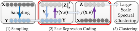
- We propose a fast regression coding (FRC) to quickly compute the codes of large-scale data points. We prove that FRC has a grouping effect that tends to group highly correlated data together.
- By using FRC, we develop an efficient RCC framework: sampling, FRC and LSSpC to solve the LSSC problem. Moreover, the complexity of RCC is O(n).
2 RelatedWorks
The subspace clustering methods have shown excellent performance in many real-world applications (also see [Vidal, 2011] for a review). In this section, we mainly review the classical coding (CCod) methods, and the large-scale spectral clustering (LSSpC) methods.
CCod usually selected the observed data matrix X itself as the dictionary in the independent and disjoint subspaces, such as LSR [Lu et al., 2012], SSC [Elhamifar and Vidal, 2013], and LRR [Liu et al., 2013]. However, this leads to the fact that the coding methods are difficult to compute the codes for the LSSC problems because they spend a lot of time to optimize the codes. In addition, many improved coding methods are proposed in the literatures, such as structured sparse subspace clustering [Li and Vidal, 2015], divide-factor-combine LRR [Talwalkar et al., 2013], and Laplacian regularized LRR [Yin et al., 2016]. However, they are still difficult to solve the LSSC problem due to the expensive inference time. Compared to CCod, our method (FRC) can quickly calculate the codes by using a non-linear projection function.
LSSpC can be roughly divided into two main ways. The first way is to reduce the computational cost of eigendecomposition over the Laplacian matrix, such as the Nystr¨ om method for the approximate eigenvectors [Fowlkes et al., 2004], and parallel eigenvalue computations in distributed systems [Chen et al., 2011]. The second way is to reduce the data size by selecting a small number of samples to replace the original data, for example, k-means methods [Yan et al., 2009], the out-of-sample data [Nie et al., 2011], and LSC [Cai and Chen, 2015]. Although those LSSpC algorithms can solve the LSSC problem, they will lead to poor results as the complex data structure easily results in an indivisible affinity matrix. Compared to LSSpC, our method fast computes the divisible codes, and preform clustering by LSC.
3 Regression Coding Clustering (RCC)
In this section, we develop an efficient Regression Coding Clustering (RCC) framework, which consists of sampling, FRC and LSSpC, to largely cluster a collection of multi-subspace data. Specifically, we formulate a fast regression coding (FRC) model to learn the non-linear function, and then adopt an analytical method and a gradient descent algorithm to solve the FRC model. The landmark-based spectral clustering (LSC) [Cai and Chen, 2015] is used to fast segment the codes of all data points computed by the function. Finally, we provide some theoretical guarantees to show that FRC recovers the subspace representations (codes) effectively.
3.1 ProblemFormulation.
To address the LSSC problem in Definition 1, we reduce the data size by selecting a small data matrix Yi ∈ Rd×mi drawn from the data matrix Xi ∈ Rd×ni in the ith subspace Si (1 ≤ i ≤ k), where mi is the number of the samples of Yi, and ri < mi ≪ ni. Then Y = [Y1 , · · · ,Yi , · · · ,Yk ] (m = ∑ki=1 mi) is used as a small dictionary, and r = ∑ki=1 ri < m = ∑ki=1 mi ≪ n = ∑ki=1 ni. In order to show the fast coding ability of the small data matrix Y, we extend the SE property [Elhamifar and Vidal, 2013] to a fast selfexpressiveness property, which is formally defined as:
Definition 2 (Fast Self-Expressiveness (FSE) Property). For the large-scale data matrix X ∈ Rd×n , there exists a non-linear function f(·; θ) ∈ Rm×n such that X = Yf(X; θ), where a small data matrix Y ∈ Rd×m is drawn from X, and the parameter θ is learned from the following system:
Remark 1: In general, the traditional coding methods consider Zii = 0 which aims to avoid the self-representation [Lu et al., 2012; Elhamifar and Vidal, 2013]. However, we use Y as a self-expressive dictionary to learn the projective function to compute the representations of the large data matrix X. Thus, Zii = 0 is not restricted in (1).
To fast train the non-linear function to approximate the codes, we exploit a three-layer neural networks (NN) as:
where g(·) is a nonlinear activation function (that is also a element-wise transformation), W1 ∈ Rh×d and W2 ∈ Rm×h are the projective weights, h is the number of hidden units. In this paper we mainly consider the tanh activation function f(a) = (ea -e-a )/(ea +e-a ), while other nonlinearities (i.e., sigmoid f(a) = 1/(1 + e-a ), rectified linear unit max(0, a), and rectifier piecewise linear units [Li et al., 2017b]) can also be used.
The Frobenius norm ‖Z‖2F in LSR has the power to capture the strong correlations in the same subspace, and does not take more time to carry out many iterations for convergence [Lu et al., 2012]. Moreover, it is used to control the over-fitting problem. To replace f(Y; θ) by (2), therefore, we propose a FRC model defined as:
In addition, data are often corrupted by noise due to measurement/process noise and collection techniques in real-world problems [Liu et al., 2013; Elhamifar and Vidal, 2013], for example, the small and independent and identically distributed (i.i.d.) Gaussian noise. In general, the Frobenius norm is used to measure the quality of approximation for fitting the Gaussian noise [Elhamifar and Vidal, 2013]. By using the Frobenius norm to penalize the noise, the problem (3) is written as the following optimization:
where α is a parameter to balance the effects of two terms.
Remark 2: In fact, when Y is selected as the dictionary, LSR also can be considered as the following problem:
Usually, it has a solution C⋆ = (YT Y+αI)-1YT X, where α is a regularization parameter. Clearly, this solution is a linear function. However, the linear projection is very limited for clustering tasks as they cannot extract more abstract and non-linear representations [Bengio et al., 2013; Li et al., 2017b]. Therefore, we train a non-linear function (2) to approximate the codes. The approximate accuracy will be studied in subsection 3.4. Moreover, the empirical evidence in Table 6 shows that our non-linear model is better than LSR.
3.2 Optimization.
The problem (4) is non-convex due to the nonlinear function g(·) in NN (2). Fortunately, NN with the suitable number 1 of hidden units can approximate any continuous function [Haykin, 2009]. Then the problem (4) can be written as:
where β is a regularization parameter. The problem (6) is solved by iteratively updating the variable Z, and the weights {W1,W2}. Thus, we first adopt the ridge regression [Hoerl and Kennard, 2000] to solve Z, and then use a gradient descent algorithm to train {W1,W2} to approximate Z. The iteration will lead to be time consuming because it needs to train {W1,W2} many times after each updating Z. Clearly, the high time cost is not beneficial to LSSC. Therefore, to avoid the iterative time cost, we use the ridge regression to solve Z without the last term of (6). The scheme is as follows:
Computing Z: Z is calculated by minimizing L without the last term of (6). By removing the last term, the problem (6) is written as the following subproblem:
1 The number of hidden units h is selected by depending on the approximating accuracy between Z and W2g(W1Y).
Algorithm 1 FRC via the gradient descent algorithm
- 1: input: data Y, the number of hidden units h, maximal training epochs Tm, regularization parameters α, β, γ, learning rate ε, and approximation accuracy ϵ.
- 2: initialize: random initializationW1, and t = 1.
- 3: compute Z⋆ by Z⋆ = (YT Y+αI)-1 YT Y.
- 4: while t < Tm and not converged do
- 5: compute H by H = g(W1Y);
- 6: updateW2 by (9);
- 7: updateW1 byW1 =W1 - ε ∂LW1,W2 ∂W1 , where ∂LW1,W2 ∂W1 is defined in (10);
- 8: check the condition: ‖Z⋆ -W2g(W1Y)‖2F /m< ϵ.
- 9: t = t + 1;
- 10: end while
- 11: return solutions W1 andW2.
Clearly, this subproblem is easily solved by a ridge regression [Hoerl and Kennard, 2000].
Updating W1 and W2: W1 and W2 are calculated by minimizing L with respect to W1 and W2, when Z is fixed. In general, the Frobenius norm is used to prevent the overfitting of weights in neural networks. So, by adding two regularization terms 2 ‖W1‖2F and ‖W2‖2F , the optimal solution is to solve the following subproblem:
where γ is a regularization parameter. The gradient descent algorithm is used to learn W1 and W2. Once the weight W1 is fixed, H = tanh(W1Y) is also determined uniquely. Then, solving W2 can be formulated as a convex optimization problem ‖Z⋆ -W2H‖2F , which has a closed-form solution:
By using a gradient descent (GD) algorithm [Li et al., 2015; Li et al., 2016] to minimize the the least squares objective in (8), deriving the gradient of W1 obtains
where ◦ denotes element-wise multiplication, 1 is an identical matrix, and 1-H◦H is the gradient of H = tanh(W1Y). The complete optimization procedure of FRC is summarized in Algorithm 1, which includes the details of updating gradients and the convergence conditions.
Time Complexity and Convergence Analysis. The computational bottlenecks of FRC lies in the matrix inversion in step 3, of which the maximum complexity is O(m3 ). Considering the cost of the gradient descent algorithm in steps
2 In order to easy understand our main idea, we do not add the regularization into the main objective function (4) as this regularization is a common trick in neural networks.
Algorithm 2 Regression Coding Clustering.
- 1: input: large-scale data Xwith k subspaces ;
- 2: select Y fromX;
- 3: solveW1 andW2 by FRC in Algorithm 1;
- 4: compute ZX by Z =W2g(W1X);
- 5: apply LSC to segment X into k subspaces by ZX;
- 6: output: segmentation of the data: X1 ,X2 , · · · ,Xk .
| Mehtods | training time | coding time |
|---|---|---|
| FRC (ours) | O(m3 +Tm(m3+ dhm + hm2 )) | O(dhn+hmn) |
| SSC [Elhamifar and Vidal, 2013] LRR [Liu et al., 2013] LSR [Lu et al., 2012] | O(0) O(0) O(0) | O(t1(d2 n2 + dn3 )) O(t2(d2 n + n3 )) O(n3 ) |
n:♯ of samples; d:♯ of dimensionality of sample; m:♯ of the selected samples; h:♯ of hidden units of non-linear function; t1, t2, Tm:♯ of the number of iterations in
l1 solver, rank-minimizer, training the non-linear function; O(0): no training time.
4-10 and the number of iterations needed to converge, the overall computational complexity of FRC is O(m3 + Tm(m3 + dhm+hm2 ))), where L ≤ 10 in this paper. The complexities of FRC and the coding methods (e.g. SSC, LRR, and LSR) are summarized in Table 1. In fact, the training complexity can be ignored due to n ≫ m. So, our coding complexity O(mn) is linear in terms of n. Thus, our method is easily scalable for computing the codes in large-scale datasets. When n = m, we can directly use LSR to obtain the codes.
The theoretical convergence of FRC is difficultly guaranteed because the gradient descent (back-propagation, BP) algorithm cannot be proved to converge [Haykin, 2009]. Fortunately, BP have been widely used in many applications as they empirically converges well in general [Haykin, 2009]. The convergence is reached when the change in objective function is below a user-defined threshold ϵ = 10-4 .
3.3 Clustering.
Our RCC procedure summarized in Algorithm 2 is available for both large and small datasets. To large datasets (e.g. MNIST, and JCNORB), we select a small data Y ∈ Rd×m from X ∈ Rd×n to train the weights W1 and W2. After training W1 and W2 by FRC, the codes ZX of X can be fast computed by f(X; {W1,W2}) in (2). We cluster ZX by employing LSC [Cai and Chen, 2015] to obtain the final results.
To small datasets (e.g. Extend-YaleB and AR), we select all data points X as Y. Similar to the SSC method, spectral clustering is applied on the affinity matrix C = |ZX| + |ZTX | to segment the data into k subspaces by NCuts [Shi and Malik, 2000]. Clearly, it cannot segment the large-scale datasets.
3.4 Theoretical Analysis.
To solve the LSSC problem, FRC trains the function (2) to approximate the codes learned by (5). In this subsection, we show an approximation condition and a grouping effect to verify that FRC is fit for large-scale subspace clustering.
Approximate the subspace representations by FRC. A sufficient condition is to show that FRC can effectively approximate the subspace representations.
| Data set | # samples | Dimension | # classes |
|---|---|---|---|
| Extend-YaleB | 2,414 | 32,256 | 38 |
| AR | 1,400 | 19,800 | 100 |
| MNIST | 70,000 | 784 | 10 |
| JCNORB | 349,920 | 2,048 | 6 |
Theorem 1 3 . Assume a large-scale set of data points X drawn from k independent subspaces {Si}ki=1 with ri bases, and a small data points Y drawn from the large data points X, where rank(X) = rank(Y) = r. For any U drawn from X, if U belongs to the neighbourhood of Y with radius ρ > 0, that is, U ∈ {P ∈ X|‖P - Y‖2F < ρ}, and
then we have ‖C⋆ - Z‖2F ≤ o (ρ), where Y† is the pseudoinverse of Y, C⋆ is the code of U learned by (5), Z = f(U; θ), f(·; θ) is a projective function (i.e. (2)), and θ is trained by the FRC problem (3).
Remark 3: The condition (11) is easily satisfied because f(·; θ) is learned from the FRC problem (3). Hence, the projective codes can approximate to the subspace representations by a first-order accuracy as long as U drawn from X is belonging to the neighbourhood of Y.
Grouping effect. The grouping effect means that the correlated data has the approximately equal coefficients, which implies these coefficients are easy to construct the similarity graph to divide the data for LSSC. We prove that FRC exhibits this grouping effect, which is stated as following:
Theorem 2. Given a data vector x ∈ Rd selected from large-scale data X, a dictionary Y ∈ Rd×m and two parameters α, β. Assume each data point of Y is normalized and x ∈ U, where U ∈ {P ∈ X|‖P - Y‖2F < ρ}. Let z = [z1, · · · , zm] = f(x; θ) be the non-linear code, where θ is trained by the FRC problem (3). If the condition (11) is satisfied, then we have
where ν = yTi yj is the dictionary correlation.
Remark 4: Theorem 2 shows that the solution is dependent correlation. If yi and yj are highly correlated (that is ν = 1), then the difference between the coefficient of yi and yj tends to be 0 due to the higher-order infinitesimal o (ρ). Hence, naturally, they will be grouped in the same cluster.
4 Experiments
In this section we evaluate our approach on four databases: Extended-YaleB 4 , AR 5 , MNIST 6 , and JCNORB 7 in Table 2.
Datasets: Extended-YaleB contains 2,414 frontal face images of 38 people. There are about 64 images for each person. AR consists of over 4,000 color images of 126 people. Each person has 26 face images taken during two sessions. We use a subset of the dataset consisting of 2,600 images from 50 male subjects and 50 female subjects. For computational efficiency, the original images of Extended-YaleB and AR were cropped and normalized to 48 × 42 and 55 × 40 pixels, respectively. Moreover, the features are reduced to 167 and 114 dimensions by PCA. MNIST has 70,000 examples with 28 × 28 pixel greyscale images of handwritten digits 0-9. JCNORB contains images of 50 toys belonging to a background and 5 generic categories: four-legged animals, human figures, airplanes, trucks, and cars. There are 349,920 training and testing examples with six classes. The original 2 × 96 × 96 images were subsampled and scaled to 2 × 32 × 32. The features are reduced to 500 dimensions by PCA.
3 The proofs of Theorems 1 and 2 are provided in https://www.researchgate.net/profile/Jun Li7
4 http://vision.ucsd.edu/ leekc/ExtYaleDatabase/ExtYaleB.html
5 http://www2.ece.ohio-state.edu/ aleix/ARdatabase.html
6 http://yann.lecun.com/exdb/mnist/
7 http://www.cs.nyu.edu/ ylclab/data/norb-v1.0/
4.1 Baselines and Evaluation Criterion.
The proposed clustering framework, RCC, employs LSC-K to segment the data points, based on the codes computed by our FRC. To evaluate the clustering performance of RCC, we compare our method with the classical coding (CCod) methods, the fast coding (FCod) methods, the large-scale spectral clustering (LSSpC) methods, and the sampling, clustering and classification (S-C-C), as well as the k-means [Cai, 2011]. Specifically, they are described as follow:
- CCod respectively uses LSR [Lu et al., 2012], SSC [Elhamifar and Vidal, 2013], and LRR [Liu et al., 2013] to calculate the codes of data samples, which are used to construct an affinity matrix, and employs NCuts to segment the data samples.
- FCod is a related method, which also learns a projective function to approximate the (sparse) codes, such as, Denoising autoencoders (DAE) 8 [Vincent et al., 2010] and predictive sparse decomposition (PSD) [Kavukcuoglu et al., 2008; Gregor and LeCun, 2010]. In reality, LSR with a small dictionary [Lu et al., 2012] becomes a linear coding function shown in Remark 2. To compare these models, they are used to fast calculate the codes in our RCC framework, and also employ LSC-K [Cai and Chen, 2015] to cluster the data points.
- LSSpC directly uses the data points to construct an similarity matrix and segment the data points. Nystr¨ om [Chen et al., 2011] finds an approximate eigendecomposition of
8 We use the codes from http-
s://github.com/kyunghyuncho/deepmat.
| Extended-YaleB | AR | |||
|---|---|---|---|---|
| ACC | NMI | ACC | NMI | |
| RCC (ours) | 66.5±1.74 | 70.5±0.79 | 82.8±0.80 | 91.1±0.36 |
| DAE [Vincent et al., 2010] | 59.6±1.25 | 61.1±0.73 | 62.3±0.95 | 70.2±0.59 |
| PSD [Gregor and LeCun, 2010] | 72.2±0.87 | 73.0±0.61 | 80.8±1.05 | 90.5±0.44 |
| LSR [Lu et al., 2012] | 67.0±1.17 | 70.7±0.51 | 83.1±1.21 | 91.3±0.28 |
| SSC [Elhamifar and Vidal, 2013] | 76.5±1.22 | 78.4±0.35 | 78.1±1.72 | 88.3±0.95 |
| LRR [Liu et al., 2013] | 67.2±0.98 | 70.4±0.55 | 82.0±1.16 | 91.3±0.51 |
| LSR-R [Cai and Chen, 2015] | 43.4±2.08 | 55.2±0.87 | 33.9±1.02 | 62.0±0.49 |
| LSR-K [Cai and Chen, 2015] | 43.4±1.21 | 54.5±0.63 | 34.4±0.72 | 62.5±0.67 |
| Nystr¨ om [Chen et al., 2011] | 24.5±1.16 | 44.2±1.02 | 61.8±2.40 | 83.0±0.90 |
| Nystr¨ omO [Chen et al., 2011] | 21.5±0.98 | 41.4±1.05 | 57.6±2.20 | 79.8±1.22 |
| k-means [Cai, 2011] | 8.6±0.55 | 10.4±0.66 | 28.0±0.98 | 58.2±0.51 |
the similarity matrix, and Nystr¨ omO [Chen et al., 2011] is constrained in the orthogonal eigenvectors. LSR-R [Cai and Chen, 2015] randomly selects a few samples as the landmarks to compute the similarity matrix, while LSR-K [Cai and Chen, 2015] uses k-means to select the landmarks.
- S-C-C follows a strategy: sampling, clustering and classification. Specifically, select+SSC (selSSC) and select+LRR (selLRR) [Wang et al., 2014] respectively use SSC and LRR to cluster the sampling data, and learn a linear classifier to segment the rest data, while SLSR, SSSC and SLRR [Peng et al., 2016] respectively cluster the sampling data based on LSR, SSC and LRR, and use SRC or CRC to classify the rest data.
The clustering quality is measured by Clustering Accuracy (ACC) and Normalized Mutual Information (NMI) [Cai and Chen, 2015] between the produced clusters and the ground truth categories. ACC and NMI both range from 0 to 1, where 1 indicates perfect matching with the true subspace distribution, whereas 0 indicates totally mismatch. To obtain reliable results, each experiment is repeated 10 times, and the final results are reported by the mean and standard deviation of ACC and NMI.
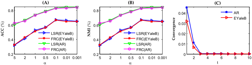
In our FRC, there are three parameters ε, α, and β. The learning rate ε, as a typical parameter in neural networks, is set to 0.0001 in all experiments. Fig. 2 (A) and (B) show ACC and NMI with different α on AR and Extend-YaleB, and the best results is shown in α = 0.1. We set α = 25 and 250 respectively for MNIST and JCNORB to obtain the best results. Due to the limited space, we do not show the varying results with different α for these two datasets. The parameter β does not affect FRC as it is solved by minimizing L without the last term of (6). In all experiments, the number of hidden units h is set to 1000, the parameter γ is set to 0.0001, tanh is voted as the activation function, and the number of training epochs Tm is less than 10.
| Extend-YaleB | AR | |||
|---|---|---|---|---|
| RCC (ours) | training 23 | coding 0.4 | training 49 | coding 0.2 |
| LSR [Lu et al., 2012] | 20 | 48 | ||
| SSC [Elhamifar and Vidal, 2013] | 56 | 72 | ||
| LRR [Liu et al., 2013] | 41 | 63 | ||
| MNIST | JCNORB | |
|---|---|---|
| RCC (ours) | 30 | 262 |
| SLSR [Peng et al., 2016] | 541 | 1365 |
| SLRR [Peng et al., 2016] | 638 | 2617 |
| SSSC [Peng et al., 2016] | 613 | 2603 |
| selSSC [Wang et al., 2014] | 469 | 3629 |
| selLRR [Wang et al., 2014] | 1569 | 4489 |
4.2 Comparison on Small-scale Datasets.
We verify that our approach (RCC) efficiently approximate the clustering results of the classical coding methods. When all samples are selected as training samples in Extended-YaleB and AR, the results are reported in Table 3. We observe that the performance of RCC is comparable to LSR as RCC trains a non-linear function to effectively approximate LSR. Moreover, RCC has a similar clustering result to other CCod methods, such as SSC and LRR. In addition, Table 3 also shows that CCod is much better than k-means and LSSpC (such as LSRR, LSR-K, Nystr¨ om and Nystr¨ omO). Clearly, this observation drives us to apply the coding methods to fast compute the codes of the data samples for LSSC.
Table 4 shows that the coding time of RCC are 0.4, and 0.2 second in Extended-YaleB and AR, which are 50 times faster than LSR, SSC and LRR at least. Hence, RCC is able to apply for large-scale datasets when we randomly select the training samples. Moreover, Fig. 2 (C) does not only show the approximation accuracy between the codes and the nonlinear function, but also illustrates that Algorithm 1 converges quickly. Although RCC spends some time to train the function, it can infer the codes in a rapid way.
4.3 Comparison on Large-scale Datasets.
It is worth noting that the CCod methods (LSR, LRR and SSC) have difficultly (or impossibly) to infer the codes in largescale datasets with over 10,000 samples. Thus, we develop FRC to fast compute the codes for large-scale clustering. For large-scale datasets, 2000 and 2400 samples are respectively selected as the training data in MNIST, and JCNORB. The clustering times and results are reported in Table 5 and Table 6, respectively. We have the following observations:
Table 6 shows that our proposed RCC outperforms all the baseline methods in the scenario of large-scale datasets. Compared to the S-C-C methods (for example, SLSR, SLRR, SSSC, selSSC, and selLRR), FRC has significantly better clustering performance, where we achieve at least 18.2% (MNIST), and 7.4% (JCNORB) improvement by ACC; and also reaches 15.2% (MNIST), and 8.8% (JCNORB) improvement by NMI.
| MNIST (2000) | JCNORB (2400) | ||
|---|---|---|---|
| ACC NMI | ACC | NMI | |
| FCod | |||
| RCC (ours) LSR [Lu et al., 2012] PSD [Gregor and LeCun, 2010] DAE [Vincent et al., 2010] | 73.6±3.79 69.6±2.15 69.8±2.35 67.3±1.03 50.1±1.79 43.7±0.38 68.9±3.71 68.6±1.67 | 32.6±1.00 31.5±0.68 29.3±2.85 26.6±2.59 | 15.4±0.66 14.5±1.56 9.7±3.06 9.4±3.28 |
| S-C-C | |||
| SLSR [Peng et al., 2016] SLRR [Peng et al., 2016] SSSC [Peng et al., 2016] selSSC [Wang et al., 2014] selLRR [Wang et al., 2014] | 54.1±1.56 48.1±0.87 50.0±3.87 49.1±2.27 54.9±1.89 49.9±1.15 55.2±1.63 54.4±2.19 55.4±5.11 52.1±2.50 | 25.4±0.67 22.9±0.22 20.9±0.46 20.6±0.67 23.4±0.30 | 6.6±0.41 5.0±0.27 2.0±0.37 2.1±0.69 4.1±0.18 6.5±2.20 7.8±0.40 7.8±0.23 |
| LSSpC | |||
| LSR-R [Cai and Chen, 2015] LSR-K [Cai and Chen, 2015] Nystr¨ om [Chen et al., 2011] Nystr¨ omO[Chen et al., 2011] | 58.5±4.19 55.8±2.65 68.3±4.99 67.7±2.29 52.7±1.46 47.4±0.38 52.1±3.48 46.9±1.49 | 24.4±0.32 24.6±0.36 25.6±0.29 27.3±0.72 | 8.6±0.30 |
| 55.3±0.06 | |||
| k-means [Cai, 2011] | 52.6±0.19 | 23.1±0.00 | 5.3±0.00 |
The fundamental reason is that the linear classifier cannot handle the complex image data in the S-C-C methods. In contrast, our method trains the non-linear function to fast capture the excellent codes of the complex image data, and then perform LSC-K. Compared to LSSpC without coding (such as LSR-R, LSR-K, Nystr¨ om, and Nystr¨ omO), RCC still shows higher ACC and NMI as RCC can learn the excellent codes of the original data points. In addition, RCC is better and faster than DAE and PSD in the FCod methods. Besides, RCC is also better than LSR as RCC trains a non-linear function.
The overall clustering time consists of the training, coding, and clustering times. RCC is faster than S-C-C since RCC can very fast infer the codes by only computing a non-linear function. As shown in Table 5, RCC is round five times faster than SLSR, SLRR, SSSC, selLRR, and selSSC. On the other hand, although the LSSpC methods are faster than RCC, their clustering results performworse than RCC. In fact, the time complexities of RCC is comparable to LSSpC as the number of data points increases. Moreover, RCC has a faster training time than other FCod methods.
5 Conclusion
To effectively solve the LSSC problem, we presented an efficient RCC framework: sampling, FRC and LSC. Firstly, a small dataset is (randomly) sampled from the large-scale data points due to the effectiveness of sampling. Secondly, based on fast self-expressiveness property, we proposed an FRC model to train a non-linear function from the sampled data for fast computing the codes of all the data points. Thirdly, the LSC method was employed to cluster the codes computed by the non-linear function. Besides, we theoretically proved that the non-linear function can approximate the codes learned from LSR by a first-order accuracy, and have a grouping effect that tends to group highly correlated data together. Extensive experimental results verified that our method can be successfully applied into the LSSC problem.
Acknowledgments
This work is supported in part by the NSF IIS award 1651902, ONR Young Investigator Award N00014-14-1-0484, and U.S. Army Research Office Young Investigator Award W911NF14-1-0218.
@inproceedings{ijcai2017p297,
  title     = {Large-scale Subspace Clustering by Fast Regression Coding},
  author    = {Li, Jun and Zhao, Handong and Tao, Zhiqiang and Fu, Yun},
  booktitle = {Proceedings of the Twenty-Sixth International Joint Conference on
               Artificial Intelligence, {IJCAI-17}},
  publisher = {International Joint Conferences on Artificial Intelligence Organization},
  editor    = {Carles Sierra},
  pages     = {2138--2144},
  year      = {2017},
  month     = {8},
  note      = {Main track},
  doi       = {10.24963/ijcai.2017/297},
  url       = {https://doi.org/10.24963/ijcai.2017/297},
}
TY - CPAPER TI - Large-scale Subspace Clustering by Fast Regression Coding AU - Li, Jun AU - Zhao, Handong AU - Tao, Zhiqiang AU - Fu, Yun T2 - Proceedings of the Twenty-Sixth International Joint Conference on Artificial Intelligence, IJCAI-17 PB - International Joint Conferences on Artificial Intelligence Organization PY - 2017 SP - 2138 EP - 2144 DO - 10.24963/ijcai.2017/297 UR - https://doi.org/10.24963/ijcai.2017/297 ER -Copied
Machine-readable versions of this paper, for tools and AI agents:





