
Integrating Specialized Classifiers Based on Continuous Time Markov Chain
Proceedings of the Twenty-Sixth International Joint Conference on Artificial Intelligence. Main track. Pages 2244-2251.
https://doi.org/10.24963/ijcai.2017/312
Keywords
- Machine Learning: Classification
- Machine Learning: Deep Learning
- Machine Learning: Ensemble Methods
Abstract
Specialized classifiers, namely those dedicated to a subset of classes, are often adopted in real-world recognition systems. However, integrating such classifiers is nontrivial. Existing methods, e.g. weighted average, usually implicitly assume that all constituents of an ensemble cover the same set of classes. Such methods can produce misleading predictions when used to combine specialized classifiers. This work explores a novel approach. Instead of combining predictions from individual classifiers directly, it first decomposes the predictions into sets of pairwise preferences, treating them as transition channels between classes, and thereon constructs a continuous-time Markov chain, and use the equilibrium distribution of this chain as the final prediction. This way allows us to form a coherent picture over all specialized predictions. On large public datasets, the proposed method obtains considerable improvement compared to mainstream ensemble methods, especially when the classifier coverage is highly unbalanced.
- [Breiman, 1996] Leo Breiman. Bagging predictors. Machine learning, 24(2):123-140, 1996.
- [Dietterich and Bakiri, 1995] Thomas G. Dietterich and Ghulum Bakiri. Solving multiclass learning problems via error-correcting output codes. Journal of artificial intelli- gence research, pages 263-286, 1995.
- [E. Mandler, 1988] J. Schurmann E. Mandler. Combining the classification results of independent classifiers based on the dempster-shafer theory of evidence. Pattern recog- nition and artificial intelligence, pages 381-393, 1988.
- [Fabian Caba Heilbron and Niebles, 2015] Bernard Ghanem Fabian Caba Heilbron, Victor Escorcia and Juan Carlos Niebles. Activitynet: A large-scale video benchmark for human activity understanding. In Proceedings of the IEEE Conference on Computer Vision and Pattern Recognition, pages 961-970, 2015.
- [Freund et al., 1996] Yoav Freund, Robert E Schapire, et al. Experiments with a new boosting algorithm. In ICML, vol- ume 96, pages 148-156, 1996.
- [He et al., 2016a] Kaiming He, Xiangyu Zhang, Shaoqing Ren, and Jian Sun. Deep residual learning for image recog- nition. In The IEEE Conference on Computer Vision and Pattern Recognition (CVPR), June 2016.
- [He et al., 2016b] Kaiming He, Xiangyu Zhang, Shaoqing Ren, and Jian Sun. Identity mappings in deep residual networks. In European Conference on Computer Vision, pages 630-645. Springer, 2016.
- [Ho, 1998] Tin Kam Ho. The random subspace method for constructing decision forests. Pattern Analysis and Ma- chine Intelligence, IEEE Transactions on, 20(8):832-844, 1998.
- [Jaakkola and Szummer, 2002] Martin Szummer Tommi Jaakkola and Martin Szummer. Partially labeled classifi- cation with markov random walks. Advances in neural information processing systems (NIPS), 14:945-952, 2002.
- [Jacobs et al., 1991] Robert A Jacobs, Michael I Jordan, Steven J Nowlan, and Geoffrey E Hinton. Adaptive mix- tures of local experts. Neural computation, 3(1):79-87, 1991.
- [Jordan and Jacobs, 1994] Michael I Jordan and Robert A Jacobs. Hierarchical mixtures of experts and the em al- gorithm. Neural computation, 6(2):181-214, 1994.
- [Karakatič and Podgorelec, 2016] Sašo Karakatič and Vili Podgorelec. Improved classification with allocation method and multiple classifiers. Information Fusion, 31:26-42, 2016.
- [Krizhevsky and Hinton, 2009] Alex Krizhevsky and Geof- frey Hinton. Learning multiple layers of features from tiny images. 2009.
- [Krizhevsky et al., 2012] Alex Krizhevsky, Ilya Sutskever, and Geoffrey E Hinton. Imagenet classification with deep convolutional neural networks. In Advances in neural in- formation processing systems, pages 1097-1105, 2012.
- [Miller, 1995] George A Miller. Wordnet: a lexical database for english. Communications of the ACM, 38(11):39-41, 1995.
- [Omari and Figueiras-Vidal, 2015] Adil Omari and Aníbal R Figueiras-Vidal. Post-aggregation of classifier ensembles. Information Fusion, 26:96-102, 2015.
- [Rogova, 1994] Galina Rogova. Combining the results of several neural network classifiers. Neural networks, 7(5):777-781, 1994.
- [Russakovsky et al., 2015] Olga Russakovsky, Jia Deng, Hao Su, Jonathan Krause, Sanjeev Satheesh, Sean Ma, Zhiheng Huang, Andrej Karpathy, Aditya Khosla, Michael Bernstein, Alexander C. Berg, and Li Fei-Fei. Ima- geNet Large Scale Visual Recognition Challenge. Inter- national Journal of Computer Vision (IJCV), 115(3):211- 252, 2015.
- [Sesmero et al., 2015] M Paz Sesmero, Juan M Alonso- Weber, German Gutierrez, Agapito Ledezma, and Araceli Sanchis. An ensemble approach of dual base learners for multi-class classification problems. Information Fusion, 24:122-136, 2015.
- [Sewell, 2011] Martin Sewell. Ensemble learning. RN, 11(02):02, 2011.
- [Sharkey, 1999] Amanda J. Sharkey, editor. Combining Ar- tificial Neural Nets: Ensemble and Modular Multi-Net Systems. Springer-Verlag New York, Inc., Secaucus, NJ, USA, 1st edition, 1999.
- [Simonyan and Zisserman, 2014] Karen Simonyan and An- drew Zisserman. Very deep convolutional networks for large-scale image recognition. arXiv preprint arXiv:1409.1556, 2014.
- [Szegedy et al., 2015] Christian Szegedy, Wei Liu, Yangqing Jia, Pierre Sermanet, Scott Reed, Dragomir Anguelov, Dumitru Erhan, Vincent Vanhoucke, and Andrew Rabi- novich. Going deeper with convolutions. In Proceedings of the IEEE Conference on Computer Vision and Pattern Recognition, pages 1-9, 2015.
- [Szegedy et al., 2016] Christian Szegedy, Sergey Ioffe, Vin- cent Vanhoucke, and Alex Alemi. Inception-v4, inception- resnet and the impact of residual connections on learning. arXiv preprint arXiv:1602.07261, 2016.
- [Tieleman and Hinton, 2012] T. Tieleman and G. Hinton. Lecture 6.5-RmsProp: Divide the gradient by a running average of its recent magnitude. COURSERA: Neural Networks for Machine Learning, 2012.
- [Wolpert, 1992] David H Wolpert. Stacked generalization. Neural networks, 5(2):241-259, 1992.
- [Woźniak et al., 2014] Michał Woźniak, Manuel Graña, and Emilio Corchado. A survey of multiple classifier systems as hybrid systems. Information Fusion, 16:3-17, 2014.
- [Xu et al., 2006] Yunpeng Xu, Xing Yi, and Changshui Zhang. A random walks method for text classification. In SDM, pages 340-347. SIAM, 2006.
References were extracted automatically from the PDF and may contain errors.
Full text extracted automatically from the PDF; figures, tables and equations may differ. The PDF is the version of record.
1 Introduction
Classifier combination is a widely used strategy for improving classification performance. Previous study along this line has resulted in a plethora of methods [Sharkey, 1999; Sewell, 2011; Wo´zniak et al., 2014]. However, with the recent rise of deep learning [Krizhevsky et al., 2012; Szegedy et al., 2015; Simonyan and Zisserman, 2014; He et al., 2016a], a question regarding the utility of classifier ensemble arises: Is it still useful to combine classifiers given the strong performance of state-of-the-art deep networks?
Real-world practice in recent years suggests a positive answer to this question. First, on a number of significant challenges, e.g. ImageNet [Russakovsky et al., 2015] and ActivityNet [Fabian Caba Heilbron and Niebles, 2015], top-ranked solutions all rely on ensembles to achieve competitive performance. For example, on ImageNet, an ensemble can often attain over 10% of relative error reduction compared to any individual classifiers, including state-of-the-art networks, e.g. Inception-ResNet [Szegedy et al., 2016]. We also observed empirically that combinations of specialized classifiers can often outperform a general classifier, sometimes by a considerable margin. Second, training a deep network usually requires a large dataset and a sheer amount of computational resources. This is not always feasible when factors like time, cost, and data availability are taken into account. Under such circumstances, there can be no other choices but to rely on existing classifiers. It is not uncommon that the classifiers from different sources cover different sets of classes. Therefore, classifier combination remains an effective method to improve performance. It may even be an indispensable part in certain real-world applications.
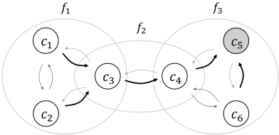
This paper proposes a novel way to integrate specialized classifiers. Instead of combining their predictions directly, we consider the procedure of reaching the final prediction as a biased random walk among classes. Specifically, we decompose each prediction into a set of pairwise preferences and then construct a continuous-time Markov chain by treating such preferences as transition channels, as shown in Figure 1. This way results in a unified picture over all specialized predictions, from which we may draw a more reliable conclusion.
We tested the proposed methods on large datasets. The results show that the presented methods can lead to further performance gains over state-of-the-art deep networks. The predictions derived from these methods are also more accurate than those based on classical combination techniques. It is also noteworthy that the presented formulations are very general and can be directly used in various contexts. For example, one can use them to combine out-of-box classifiers trained for different sets of classes to support a more general application, without re-training.
2 RelatedWork
Extensive study on classifier combination for decades had led to a plethora of methods. See [Sharkey, 1999; Sewell, 2011; Wo´zniak et al., 2014] for more comprehensive reviews. In general, existing methods fall into two categories: ensemble methods and modular methods. Specifically, ensemble methods combine a set of classifiers that work with the same set of classes; while modular methods take advantage of domainspecific knowledges to divide the classification task into subtasks, each accomplished by a specialized expert, e.g. one expert classifies flowers, while another one differentiates between animals.
Designs of ensemble methods usually revolve around two desiderata: accuracy and diversity. To be more specific, on one hand, individual classifiers should yield reasonable predictions; on the other hand, different classifiers should be complementary to each other, such that the combination of their predictions can hopefully result in improved accuracy. Methods that are widely used for constructing diverse ensembles include Bagging [Breiman, 1996], Adaboost [Freund et al., 1996], and Random subspace [Ho, 1998], etc. The way to combine individual predictions is another focus of the research along this line. Combination schemes explored in previous work range from simple aggregation rules such as majority voting, to sophisticated models, such as stacking [Wolpert, 1992], combination based on the DempsterShafer theory [E. Mandler, 1988; Rogova, 1994], and errorcorrecting output coding [Dietterich and Bakiri, 1995].
Modular methods adopt the divide-and-conquer strategy. Particularly, they decompose the original problem into modules, and combine their results based on the structures among them. Relations among modules can be either cooperative, i.e. all modules contribute to the final prediction, or competitive, i.e. each module has its own realm. In former cases, simple rules such as weighted voting are often used; while for the latter, a particular module needs to be chosen in advance to make the prediction. For example, Mixture of Experts [Jacobs et al., 1991; Jordan and Jacobs, 1994] makes this choice via a gating network.
In recent years, classifier combination remains under active research [Karakatiˇc and Podgorelec, 2016; Omari and Figueiras-Vidal, 2015; Sesmero et al., 2015], which focus primarily on the construction of complementary classifiers or adaptive weighed combination. These methods generally require all constituent classifiers to be aware of all classes, and thus cannot be directly applied for integrating specialized classifiers.
Continuous Time Markov Chain (CTMC) based ensemble, which we propose in this paper, makes no distinction between ensemble or modular methods. It is a very flexible framework that can coherently incorporate both general classifiers, i.e. those covering the all classes, and specialized classifiers, i.e. those working with only a subset of classes, into a unified formulation. Here, classifiers can overlap, and each class can be covered by a different number of classifiers. Compared to existing methods, it has two key advantages: (1) It takes into account the relations among predictions when integrating them as well as the different coverage of specialized classifiers. In this way, it can produce more reliable predictions when the ensemble is diverse or unbalanced. (2) It does not rely on any assumptions of the relations among classifiers (e.g. there is no requirements that they cover disjoint groups of classes or they form a hierarchy, etc.). This flexibility makes it applicable to a wide range of applications and real-world settings.
It is worth noting that use of stochastic processes has been explored in different machine learning areas. For example, some semi-supervised learning methods [Jaakkola and Szummer, 2002; Xu et al., 2006] rely on Markov random walk for label propagation. Their motivation and task, however, are fundamentally different from our work.
3 Classifier Integration Based on CTMC
We consider the task of combining multiple classifiers to make predictions. Suppose we have M classes denoted by c1, . . . , cM, and K classifiers, denoted by f1, . . . , fK. Each classifier may cover all M classes or just a small subset thereof. Particularly, the subset of classes that fk works with is given by {ci}i∈Ik , where Ik is a set of indexes. When |Ik| = M, i.e. fk covers all classes, fk is called a general classifier, otherwise, it is called a specialized classifier.
Given a sample x, fk yields an |Ik|-dimensional prediction vector pk ∈ R|Ik| , in which the entry pk(i) with i ∈ Ik is the probability of sample x belonging to class ci from the view of classifier fk. Various ways can be used to turn the output of a classifier into such a prediction vector. In the simplest case, where a classifier only yields a class label, pk can be constructed as the indicator vector of the predicted class. If a classifier produces scores, e.g. SVM, one can turn the scores into a probability vector via a softmax transform. A variety of other classifiers, e.g. deep networks with softmax output, can directly yield the prediction vectors by design.
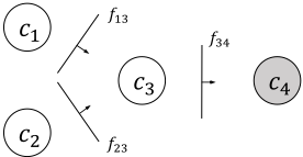
Challenges arise when combining outputs from specialized classifiers. First, a specialized classifier, when presented with a sample out of its scope, yields misleading predictions. For instance, a classifier for flower recognition would consider an apple as a certain type of flower. Second, when the coverage of classifiers is unbalanced, i.e. some classes are covered by more classifiers than others, the overall prediction may favor classes that are heavily covered. Figure 2 shows an example where the majority voting yields a wrong prediction when individual classifiers predict correctly.
3.1 Continuous-Time Markov Chains
We develop a novel methodology to effectively combine specialized classifiers based on a Continuous-Time Markov Chain (CTMC) over all classes. In this section, we review some basic properties of CTMC. Formally, a homogeneous CTMC is a stochastic process characterized by a transition rate matrix Q, where qij = Q(i, j) is the transition rate from state i to j when i ̸= j, and -qii is the parameter associated with the exponentially distributed sojourn time in state i.
The dynamic of the process can be understood in terms of alarm clocks. When the chain enters state i, independent alarm clocks are placed at all other states. The clock in state j will ring after an exponentially distributed time interval with parameter qij. When the first clock rings, the chain goes to that state, discards all alarm clocks and repeats. Hence, it is more likely to transit to a state j with larger qij value, as the average waiting time 1/qij is shorter. Since the sojourn time in state i is the minimum of a set of exponentially distributed random variables with parameters {qij : j ̸= i}, it must be an exponential random variable with parameter ∑j̸=i qij . Thus,
So, to construct a CTMC, we only need to specify the set of transition rates between different states.
When the chain is ergodic, P (Xt) will converge to an equilibrium distribution π, which, from an intuitive standpoint, reflects which states it is likely to reach in the long run. π does not depend on the initial distribution, and it is related to the transition rate matrix Q by the stationary condition:
Equation (2) together with the normalization constraint
where 1 is an all-one vector, uniquely determines the stationary probability vector π. Note that once the Q is constructed, π can be efficiently solved by most linear algebra libraries.
3.2 CTMC for Integrating Predictions
The basic idea to integrate specialized predictions is to consider the procedure of reaching the overall prediction as a stochastic process, where one can walk from one class to another, following the preferences conveyed by individual predictions. One naive implementation of this idea is by tracing.
𝑐𝑖
𝐩𝑘 𝑖 𝐩𝑘 𝑗
𝑐𝑗
(a)
Specifically, given a sample x, the classifier fk assigns it to a class ci. From this prediction, one can derive |Ik| - 1 preferences, given by {cj → ci : ∀j ∈ Ik\{i}}, meaning that the classifier prefers ci to all other classes in its domain Ik. Take the example in Figure 2 for instance, the classifiers f13, f23 and f34 together result in three preferences: c1 → c3, c2 → c3, and c3 → c4. Following these preferences, one would eventually reach the ground-truth class c4 and stay there, regardless of which class it begins with.
Ideally, when the preferences derived from all classifiers are consistent with each other, it is not difficult to reach a overall prediction by tracing the preferences. However, realworld situations are often more complicated, and individual classifiers may produce contradicting predictions. Besides, this tracing algorithm also discards the rich information in the prediction vector, i.e. those relative preferences between any pair of classes in the domain. To effectively handle such issues, a more sophisticated scheme is needed. Our approach is to generalize this deterministic tracing algorithm into a CTMC, where one may walk back and forth between classes guided by the preferences, and we rely on the equilibrium distribution to make the final predictions.
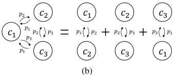
We model the pairwise preferences by CTMCs with two states. Given a sample x, denote the prediction vector from classifier fk by pk. For class ci and cj where i, j ∈ Ik, i ̸= j, we build a chain using the prediction values pk(i) and pk(j) as transition rates, which is shown in Figure 3 (a). Exploiting Equation (1), the transition rate matrix Q can be written as
We can see that (pk(i), pk(j)) is a solution to the stationary condition (2). Thus, the stationary distribution for this chain reflects the relative preference of fk on these two classes.
Combining all the (|Ik| 2 ) preferences into one chain, we can construct a CTMC for classifier fk. The state space consists of all the classes that it covers, and the transition rate from class ci to cj is set to the predicted probability for cj. One example with three classes {c1, c2, c3} and pk = (p1, p2, p3) is illustrated in Figure 3 (b). It is easy to see that the transition rate matrix can be written concisely as
where I is the identity matrix. Note that the prediction vector pk itself is the solution to the stationary condition (2), as
This consistency indicates that merging small chains into a large one is a reasonable strategy for combining preferences.
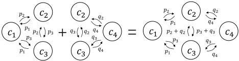
Next, we combine all the chains from different classifiers by superposition, resulting in a chain over all classes, i.e., the union of individual state spaces. In the resultant chain, the transition rates from ci to cj are the sum of all the rates defined for the pair. This process is illustrated in Figure 4. The reason for using the sum operator can be seen from the alarm clock analogy. The channel from state i to state j is set with multiple alarm clocks, and the chain transits from state i to j if any of the clocks rings. This is equivalent to set only one alarm clock who will ring after an exponentially distributed time with parameter being the sum of parameters for individual clocks. Overall, the transition rate matrix Q for the final CTMC can be written as:
Here, Sij = {k : i ∈ Ik and j ∈ Ik} refers to the index set of classifiers that cover both ci and cj. Given a sample, one can construct Q and solve the equilibrium distribution π as the final prediction. In this prediction, the most likely class label is ˆi = argmaxi π(i). Let's revisit the example in Figure 2. For this case, the transition rate matrix is given by
Then the prediction is (0, 0, 0, 1), as expected.
3.3 Properties of CTMC Formulation
First, we show that the CTMC method is applicable to a reasonable configuration of specialized classifiers. We say a set of classifiers is connected, if the graph representation of the constructed CTMC described in Section 3.2 is connected.
Proposition 1. If the classifiers in the ensemble is connected, covers all the classes when combined, and the probabilistic predictions are positive (i.e. predicting non-zero probabilities on all classes that they cover). Then the constructed CTMC is ergodic, and thus CTMC ensemble is applicable and will output a unique prediction.
Proof. The number of states is finite. To show the constructed CTMC is ergodic, it suffices to show that it is irreducible. From the construction of CTMC for each classifier (Figure 3), we know that classes belong to one classifier communicates with each other. Hence, if the classifiers are connected, then all the classes communicate with each other, and thus the irreducibility follows.
This is a mild condition. For example, it is satisfied for all those classifiers relying on a softmax transform to produce a probabilistic output. The following proposition characterizes the behavior of the CTMC ensemble.
Proposition 2. Given a transition rate matrix Q defined by Equation (7), the overall prediction π has
Here, Fi refers to the set of all classifiers that cover ci.
Proof. Let aki = I(i ∈ Ik), then qij can be rewritten as
Here, we utilize a fact akiakj = aki when i = j. Hence, πQ can be expanded into
With πQ = 0, we then obtain
Swapping i and j results in Equation (9).
Proposition 2 shows that π(i) is a weighted combination of pk(i), the corresponding entry in the predictions from the classifiers that cover ci. Here, the combination weight ωk = ∑j∈Ik π(j), which equals the total probability mass that falls in its domain Ik, can be interpreted as the relevance of the classifier fk to the given sample. Note that π and ωk are mutually dependent. The optimal π can be considered as the fixed point of Equation (9), where the classifier relevances agree with the overall prediction. Under the special setting when all classifiers cover the same set of classes, we have:
Corollary 1. If every classifier covers the entire class space, then π equals the average of individual predictions,
This corollary follows immediately from Proposition 2. In particular, ωk = 1 for each k in this case. The next corollary demonstrates the power in stitching specialized classifiers.
Corollary 2. In Proposition 1, if all specialized classifiers are obtained by first restricting results from one given general classifier into their domain and then rescaling properly, then the output of CTMC exactly recovers this general classifier.
Proof. FromProposition 2, we know that the prediction from the general classifier is a solution. This is because in Equation 9, by the construction of specialized classifiers, we have π(i) = ωkpk(i) for all i and k. Then by Proposition 1, it is the unique solution.
For example in Figure 4, suppose that the two prediction vectors are (p1, p2, p3) = (0.7, 0.1, 0.2) and (q2, q3, q4) = (0.2, 0.4, 0.4). On their shared classes c2 and c3, the relative preferences are consistent, i.e. p2 : p3 = q2 : q3 = 1 : 2. The output of CTMC is (7, 1, 2, 2)/12. We can verify that the two predictions are the restricted version of the output. This shows that CTMC ensemble can find a coherent global picture if all local information collected from specialized classifiers do not contradict with each other.
4 Experiment
We tested the proposed method in comparison with mainstream baselines on two commonly used benchmarks, ILSVRC 2012 [Russakovsky et al., 2015], and CIFAR100 [Krizhevsky and Hinton, 2009]. The ILSVRC benchmark is constructed based on ImageNet, which contains 1.2M training images in 1000 classes, and 50K validation images for testing. The CIFAR-100 dataset consists of 60K images in 100 classes, of which 50K are for training and the other 10K are for testing.
The base classifiers used in our experiments are all deep Convolutional Neural Networks (CNNs), which all have a softmax layer on top of the final representations, and thus can directly output the probabilistic prediction vectors. Particularly, three network architectures are used in our experiments, namely ResNet-56 [He et al., 2016a], pre-activation ResNet101 [He et al., 2016b], and Inception-ResNet-v2 [Szegedy et al., 2016]. In this way, we can see how well the proposed method can work with different models.
We compared with several commonly used methods for classifier combination: (1) vote: each classifier votes for the class with highest probability, and choose the smaller index if there is a tie; (2) mean: averaging the prediction scores from all individual classifiers as output; (3) m-mean: multiplicityaware mean, where the prediction scores on individual classes are averages over only those covering classifiers; (4) prod: geometric mean of the prediction scores from all individual classifiers; (5) m-prod: multiplicity-aware product, where the geometric mean of prediction scores for each class is taken over only the covering classifiers. Here, m-mean and m-prod are natural way to mitigate the effect of unbalanced classifier coverage. Following the common practice, we measure the performances by top-1 and top-5 error rates.
4.1 Combining Specialized Classifiers
The primary goal of this work is to develop an effective approach to combining specialized classifiers, i.e. those that cover subsets of classes. The first experiment is to assess the effectiveness of the CTMC method on this task, in comparison with the baseline methods.
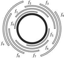
On ILSVRC We first conducted the experiment on ILSVRC. Specifically, for ILSVRC, we train 10 specialized classifiers f0, . . . , f9, each covering 300 classes. Adjacent classifiers, i.e. fk and fk+1 have 200 classes in common, as shown in Figure 5. For this experiment, we used a trimmed down version of Inception-ResNet-v2 [Szegedy et al., 2016] 1 . We followed the standard practice to train the networks, using random-crop augmentation, RMSProp [Tieleman and Hinton, 2012] with decay 0.9 and ϵ = 1.0, weight decay 0.0005, and batch size 512. The learning rate was initialized to 0.45 and scaled down by a factor 0.1 per 120K iterations. All experiments were terminated at iteration 250K to avoid overfitting.
Results obtained by combining different subsets of these specialized classifiers are shown in Table 1. For the first two rows of the table, the classifiers in the subset {f0, f2, . . . , f8} or {f1, f3, . . . , f9} are only minimally overlapped to form a connected graph, which establishes the basic performance. For the rows below, we gradually incorporate additional classifiers to increase the overlap.
From the results, we observed: (1) m-mean and m-prod, takes into account the factor of multiplicity under the condition of unbalanced coverage, yields better results than naive vote, mean and prod. Nevertheless, the CTMC method consistently outperforms all baseline methods, by considerable margins w.r.t. relative reduction of error rates compared to best baselines. (2) When increasing the number of classifiers and particularly the overlaps among them, we can observe steady improvement of the performance. (3) By combining all 10 specialized classifiers with the CTMC method, we obtained a top-1 error at 22.480% and top-5 error at 6.676%. To put the results into perspective, we also trained a general classifier using the same network structure and hyperparameters, which yields a top-1 error 24.542% and a top-5 error 7.224%. The relative reduction of top-1 and top-5 error rates are respectively 8.4% and 8.2%. This is a notable performance gain, considering the baseline was already very strong. This also suggests that combining specialized classifier is a viable way to boost performance.
1 We used a trimmed down version, so it fits our computational budget to train 10 networks. This version contains 3, 6, 3 blocks in A, B, and C regions as compared to original's 5, 10, 5.
| Classifier Set | Top-1 Error (%) | Top-5 Error (%) | ||||||||||
|---|---|---|---|---|---|---|---|---|---|---|---|---|
| vote | mean | m-mean | prod | m-prod | CTMC | vote | mean | m-mean | prod | m-prod | CTMC | |
| {f0, f2, f4, f6, f8} {f1, f3, f5, f7, f9} | 61.298 | 37.042 | 28.286 | 29.592 | 28.350 | 25.322 | 15.962 | 12.332 | 11.734 | 13.376 | 11.144 | 7.952 |
| 57.138 | 34.746 | 27.878 | 29.342 | 27.898 | 24.992 | 16.052 | 12.742 | 12.078 | 12.600 | 10.686 | 7.718 | |
| {f0, f2, f4, f6, f8} ∪ {f1} | 51.060 | 33.664 | 27.504 | 29.294 | 27.526 | 24.518 | 19.706 | 12.148 | 11.508 | 12.964 | 10.536 | 7.696 |
| {f0, f2, f4, f6, f8} ∪ {f1, f3} | 47.436 | 35.752 | 26.574 | 28.670 | 26.622 | 24.156 | 23.898 | 11.806 | 11.046 | 12.924 | 10.050 | 7.528 |
| {f0, f2, f4, f6, f8} ∪ {f1, f3, f5} | 43.172 | 34.070 | 25.912 | 27.586 | 25.832 | 23.506 | 22.020 | 11.096 | 10.620 | 12.326 | 9.634 | 7.206 |
| {f0, f2, f4, f6, f8} ∪ {f1, f3, f5, f7} | 37.300 | 28.892 | 25.008 | 25.060 | 24.828 | 22.842 | 14.856 | 10.334 | 10.136 | 9.954 | 9.206 | 6.886 |
| {f0, f1, f2, f3, f4, f5, f6, f7, f8, f9} | 30.498 | 24.530 | 24.530 | 24.258 | 24.258 | 22.480 | 14.172 | 10.014 | 10.014 | 8.548 | 8.548 | 6.676 |
| Classifier Set | Top-5 Error (%) | |||||||||||
|---|---|---|---|---|---|---|---|---|---|---|---|---|
| vote | mean | Top-1 m-mean | Error (%) prod | m-prod | CTMC | vote | mean | m-mean | prod | m-prod | CTMC | |
| {g0, g5, g10, g15} | 74.60 | 58.04 | 49.59 | 49.95 | 49.68 | 45.51 | 25.82 | 21.83 | 21.48 | 22.31 | 21.39 | 16.64 |
| {g1, g6, g11, g16} | 74.73 | 55.87 | 49.46 | 50.04 | 49.55 | 43.94 | 26.05 | 21.99 | 21.76 | 22.27 | 21.24 | 15.91 |
| {g2, g7, g12, g17} | 74.43 | 54.07 | 50.47 | 51.11 | 50.62 | 46.26 | 26.33 | 22.34 | 22.11 | 22.83 | 21.68 | 17.47 |
| {g3, g8, g13, g18} | 76.06 | 56.66 | 47.96 | 48.36 | 48.03 | 43.76 | 25.60 | 21.74 | 21.43 | 22.17 | 21.32 | 16.86 |
| {g4, g9, g14, g19} | 73.67 | 54.73 | 49.82 | 50.25 | 49.91 | 46.97 | 25.51 | 22.19 | 21.97 | 22.87 | 22.13 | 17.75 |
| {g0, g4, g8, g12, g16} | 65.42 | 55.93 | 44.67 | 45.56 | 44.74 | 41.01 | 23.56 | 21.16 | 20.31 | 21.31 | 19.05 | 15.29 |
| {g1, g5, g9, g13, g17} | 64.94 | 55.53 | 48.49 | 49.43 | 48.49 | 44.73 | 22.53 | 20.98 | 20.80 | 23.75 | 21.39 | 17.09 |
| {g2, g6, g10, g14, g18} | 65.39 | 53.66 | 46.69 | 48.37 | 47.03 | 43.21 | 22.87 | 21.39 | 21.22 | 24.10 | 21.59 | 16.72 |
| {g3, g7, g11, g15, g19} | 67.19 | 54.86 | 43.66 | 44.64 | 43.69 | 40.88 | 23.10 | 21.30 | 20.79 | 22.04 | 19.80 | 15.78 |
| {g0, g3, g6, g9, g12, g15, g18} | 54.73 | 41.63 | 40.73 | 41.23 | 41.05 | 39.82 | 21.70 | 19.15 | 18.80 | 18.47 | 18.16 | 15.83 |
| {g1, g4, g7, g10, g13, g16, g19} | 51.86 | 41.60 | 40.66 | 41.16 | 41.00 | 38.67 | 21.58 | 19.46 | 19.09 | 19.05 | 18.83 | 15.52 |
| {g2, g5, g8, g11, g14, g17} | 56.20 | 48.09 | 44.25 | 45.77 | 44.58 | 40.98 | 23.11 | 20.59 | 20.41 | 22.77 | 20.29 | 16.30 |
| {g0, g2, g4, g6, g8, g10, g12, g14, g16, g18} | 44.81 | 38.30 | 38.30 | 38.93 | 38.93 | 35.81 | 20.70 | 17.54 | 17.54 | 16.44 | 16.44 | 13.18 |
| {g1, g3, g4, g6, g9, g11, g13, g15, g17, g19} | 44.37 | 37.83 | 37.83 | 38.31 | 38.31 | 35.94 | 20.10 | 17.63 | 17.63 | 16.74 | 16.74 | 13.89 |
| {g0, g1, g2, g3, g4, g5, g6, g7, g8, . . . , g19} | 37.65 | 35.16 | 35.16 | 35.64 | 35.64 | 32.42 | 16.45 | 14.94 | 14.94 | 14.36 | 14.36 | 10.98 |
| Classifier Set | Top-1 Error (%) | Top-5 Error | ||||||||||
|---|---|---|---|---|---|---|---|---|---|---|---|---|
| vote | mean | m-mean | prod | m-prod | CTMC | vote | mean | m-mean | (%) prod | m-prod | CTMC | |
| {h0} | 22.066 | 22.066 | 22.066 | 22.066 | 22.066 | 22.066 | 21.998 | 6.146 | 6.146 | 6.146 | 6.146 | 6.146 |
| {h0} ∪ R | 22.462 | 22.092 | 22.092 | 21.820 | 21.820 | 21.836 | 16.540 | 8.356 | 8.356 | 6.404 | 6.404 | 5.972 |
| {h0} ∪ S | 25.240 | 23.278 | 23.278 | 21.782 | 21.782 | 21.708 | 22.600 | 15.292 | 15.292 | 7.670 | 7.670 | 6.108 |
| {h0} ∪ U | 43.382 | 31.564 | 23.974 | 21.792 | 21.488 | 21.308 | 25.912 | 16.532 | 15.196 | 9.948 | 8.794 | 5.802 |
| {h1} | 22.066 | 22.066 | 22.066 | 22.066 | 22.066 | 22.066 | 22.006 | 6.050 | 6.050 | 6.050 | 6.050 | 6.050 |
| {h1} ∪ R | 22.526 | 22.176 | 22.176 | 21.980 | 21.980 | 21.918 | 16.630 | 8.304 | 8.304 | 6.290 | 6.290 | 5.966 |
| {h1} ∪ S | 25.162 | 23.026 | 23.026 | 21.628 | 21.628 | 21.584 | 22.554 | 15.292 | 15.292 | 7.580 | 7.580 | 5.990 |
| {h1} ∪ U | 43.304 | 31.522 | 23.882 | 21.740 | 21.484 | 21.222 | 25.928 | 16.486 | 15.126 | 9.918 | 8.758 | 5.730 |
| {h2} | 21.980 | 21.980 | 21.980 | 21.980 | 21.980 | 21.980 | 21.914 | 6.094 | 6.094 | 6.094 | 6.094 | 6.094 |
| {h2} ∪ R | 22.446 | 22.074 | 22.074 | 21.886 | 21.886 | 21.820 | 16.534 | 8.330 | 8.330 | 6.352 | 6.352 | 5.982 |
| {h2} ∪ S | 25.210 | 23.126 | 23.126 | 21.648 | 21.648 | 21.542 | 22.552 | 15.290 | 15.290 | 7.552 | 7.552 | 5.942 |
| {h2} ∪ U | 43.326 | 31.528 | 23.982 | 21.774 | 21.468 | 21.156 | 25.882 | 16.472 | 15.076 | 9.922 | 8.760 | 5.752 |
| {h0, h1, h2} | 21.518 | 21.520 | 21.520 | 21.526 | 21.526 | 21.520 | 18.002 | 5.806 | 5.806 | 5.834 | 5.834 | 5.806 |
| {h0, h1, h2} ∪ R | 21.464 | 21.480 | 21.480 | 21.490 | 21.490 | 21.448 | 14.022 | 7.398 | 7.398 | 5.808 | 5.808 | 5.706 |
| {h0, h1, h2} ∪ S | 21.334 | 21.414 | 21.414 | 21.232 | 21.232 | 21.140 | 18.200 | 11.842 | 11.842 | 5.922 | 5.922 | 5.678 |
| {h0, h1, h2} ∪ U | 22.838 | 22.502 | 21.672 | 21.222 | 21.086 | 21.000 | 17.294 | 13.412 | 12.678 | 6.730 | 6.462 | 5.588 |
| R∪S ∪U | 48.932 | 34.850 | 26.444 | 27.490 | 26.350 | 22.222 | 25.940 | 12.832 | 11.612 | 12.588 | 10.996 | 6.070 |
| {h0, h1, h2} ∪R∪S ∪U | 21.854 | 21.758 | 21.262 | 21.180 | 21.048 | 20.972 | 14.598 | 9.884 | 9.464 | 6.462 | 6.200 | 5.488 |
On CIFAR-100 On CIFAR-100, we adopted different settings, as this dataset differs significantly from ImageNet. Specifically, we trained 20 specialized classifiers g0, . . . , g19, each covering 30 classes, and adjacent classifiers have 25 classes in common. As the image size here is much smaller (32 × 32), it suffices to use ResNet-56 as the base network. We followed the common practice to train the networks: data augmentation with random crop, SGD with momentum 0.9 and batch size 128, learning rates initialized to 0.1 and scaled down by 0.1 per 45K iterations, and weight decay 0.0005.
Table 2 shows the top-1 error rates obtained by combining different subsets of classifiers using different methods. We observed similar trends on CIFAR-100: CTMC method outperforms baseline methods consistently and significantly. Also, the performance generally improves as we increase the size of the ensemble and thus the overlap among classes (see the rows from top to bottom). Again, we trained a general classifier, which yields a top-1 error rate at 35.51%. The best error rate from an CTMC ensemble of specialized classifier is 32.42%, about 8.7% of relative reduction. However, we should also note that this reduction is achieved by combining many specialized classifiers. As shown in Table 2, when the minimal set of classifiers are combined, i.e. 4 specialized classifiers as in the first table block. the performance is not yet comparable to a well-trained general classifier. Albeit it defeats all other combining methods in the same table.
4.2 Ensemble Augmentation
We have seen that CTMC provides an effective means to combine specialized classifiers. In the following experiments, we study (1) whether we can obtain further performance gains by incorporating both general and specialized classifiers, and (2) if this is the case, what are the more effective strategies to configure a specialized ensemble.
We conducted the experiments on ILSVRC, and considered three configurations to generate specialized classifiers: (1) Random split. This baseline strategy randomly evenly splits the 1000 classes into 12 groups, and trains 12 specialized classifiers, each for one group. (2) Synset split. Each class in ILSVRC corresponds to a synset, which is a node in the wordnet hierarchy [Miller, 1995]. Therefore, we can exploit this hierarchical structure to group the classes, so that semantically related classes are brought together. Walking down along the hierarchy until reaching the nodes with moderate sub-tree sizes, we obtain 12 groups, which are listed below together with the number of classes contained therein: structures (55), materials (56), things (114), devices (122), homeware (106), vehicles (68), domestic (121), invertebrate (61), poultry (59), mammals (97), mollusc (60), and others (81). (3) Unbalanced. Both splits above use disjoint groups, and therefore each class will be covered by two classes (one general and one group-specific). In this split, we consider a setting with unbalanced coverage. Particularly, we select two large synset nodes, instrumentality (348) and animals (398), 20 small synsets, whose sizes are around 30, and 16 tiny synsets, whose sizes are below 10. These new synsets together with the 12 synsets in the synset split above result in a collection of 50 groups of classes. These groups may overlap with each other, and their sizes range from 4 to 398.
In the end, number of classes covered by 1/2/3/4 classifiers is 130/297/487/86.
In this experiment, we trained 3 general classifiers h0, h1 and h2, and multiple specialized classifiers, each for a group in the splits introduced above. For all these classifiers, including both the specialized classifiers and the general classifiers, we adopt the same pre-activation ResNet-101 architecture, modulo the difference in the last fully-connected layer, which is class number dependent. One same pre-trained model is used for the initialization. This setting is different from the ILSVRC experiment in Section 4.1 because the specialized classifiers in this experiment are finetuned from a well-trained general classifier; while those in the previous experiment are trained from scratch. Specifically, the training uses SGD with momentum 0.9 and weight decay 0.0005. Batch size is set to 200 for groups with over 50 classes or 128 for those smaller.
From the results shown in Table 3, we observed: (1) The CTMC method outperforms other combination methods in almost all settings. (2) The CTMC method generally obtains performance improvement when adding specialized methods, no matter whether the coverage is balanced or unbalanced. Other methods, including m-mean and m-prod, will see a significant performance degradation under the unbalanced condition. This clearly suggests a consistent reliability of the CTMC method. (3) The unbalanced setting which involves specialized classifiers trained on groups of different sizes yields the most significant gains using CTMC. This demonstrates the strength of the CTMC method in integrating very complex classifier configurations. Other methods all fail in such setting, resulting in performances even worse than the baseline. (4) If we remove the general classifier from the ensemble, the error rate sees a sharp rise for baseline methods, while for CTMC, the increase of error is quite moderate.
5 Conclusion
We presented a novel method for combining specialized classifiers based on the Continuous-Time Markov Chains (CTMC), which can reason about the relations among preferences conveyed by individual predictions, instead of just simply combining them. This allows it to work with diverse ensembles and the cases with unbalanced coverage.
We compared it with commonly used methods on two public benchmarks, ILSVRC and CIFAR-100. The proposed method consistent outperforms other methods under different settings. Especially when the ensemble is diverse and has unbalanced coverage, other methods failed (performing worse than a general classifier) while the CTMC method continues to bring performance improvement. These results clearly demonstrated the merits of the CTMC method - competitive performance and high reliability in complicated situations.
Acknowledgements
This work is partially supported by the Big Data Collaboration Research grant from SenseTime Group (CUHK Agreement No. TS1610626) and the General Research Fund (GRF) of Hong Kong (No. 14236516). We would like to thank Xingcheng Zhang for the artistic drawing of Figure 5.
@inproceedings{ijcai2017p312,
  title     = {Integrating Specialized Classifiers Based on Continuous Time Markov Chain},
  author    = {Li, Zhizhong and Lin, Dahua},
  booktitle = {Proceedings of the Twenty-Sixth International Joint Conference on
               Artificial Intelligence, {IJCAI-17}},
  publisher = {International Joint Conferences on Artificial Intelligence Organization},
  editor    = {Carles Sierra},
  pages     = {2244--2251},
  year      = {2017},
  month     = {8},
  note      = {Main track},
  doi       = {10.24963/ijcai.2017/312},
  url       = {https://doi.org/10.24963/ijcai.2017/312},
}
TY - CPAPER TI - Integrating Specialized Classifiers Based on Continuous Time Markov Chain AU - Li, Zhizhong AU - Lin, Dahua T2 - Proceedings of the Twenty-Sixth International Joint Conference on Artificial Intelligence, IJCAI-17 PB - International Joint Conferences on Artificial Intelligence Organization PY - 2017 SP - 2244 EP - 2251 DO - 10.24963/ijcai.2017/312 UR - https://doi.org/10.24963/ijcai.2017/312 ER -Copied
Machine-readable versions of this paper, for tools and AI agents:





