
Unsupervised Learning of Scene Flow Estimation Fusing with Local Rigidity
Proceedings of the Twenty-Eighth International Joint Conference on Artificial Intelligence. Main track. Pages 876-882.
https://doi.org/10.24963/ijcai.2019/123
Keywords
- Computer Vision: Computer Vision
- Computer Vision: 2D and 3D Computer Vision
Abstract
Scene flow estimation in the dynamic scene remains a challenging task. Computing scene flow by a combination of 2D optical flow and depth has shown to be considerably faster with acceptable performance. In this work, we present a unified framework for joint unsupervised learning of stereo depth and optical flow with explicit local rigidity to estimate scene flow. We estimate camera motion directly by a Perspective-n-Point method from the optical flow and depth predictions, with RANSAC outlier rejection scheme. In order to disambiguate the object motion and the camera motion in the scene, we distinguish the rigid region by the re-project error and the photometric similarity. By joint learning with the local rigidity, both depth and optical networks can be refined. This framework boosts all four tasks: depth, optical flow, camera motion estimation, and object motion segmentation. Through the evaluation on the KITTI benchmark, we show that the proposed framework achieves state-of-the-art results amongst unsupervised methods. Our models and code are available at https://github.com/lliuz/unrigidflow.
- [Basha et al., 2013] Tali Basha, Yael Moses, and Nahum Kiryati. Multi-view scene flow estimation: A view cen- tered variational approach. IJCV, 101(1):6-21, 2013.
- [Chang and Chen, 2018] Jia-Ren Chang and Yong-Sheng Chen. Pyramid stereo matching network. In CVPR, 2018.
- [Eigen et al., 2014] David Eigen, Christian Puhrsch, and Rob Fergus. Depth map prediction from a single image using a multi-scale deep network. In NIPS, 2014.
- [Fischler and Bolles, 1981] Martin A. Fischler and Robert C. Bolles. Random sample consensus: A paradigm for model fitting with applications to image analysis and automated cartography. Commun. ACM, 24(6):381-395, 1981.
- [Geiger et al., 2012] Andreas Geiger, Philip Lenz, and Raquel Urtasun. Are we ready for autonomous driving? the kitti vision benchmark suite. In CVPR, 2012.
- [Geiger et al., 2013] Andreas Geiger, Philip Lenz, Christoph Stiller, and Raquel Urtasun. Vision meets robotics: The kitti dataset. IJRR, 2013.
- [Godard et al., 2017] Clément Godard, Oisin Mac Aodha, and Gabriel J Brostow. Unsupervised monocular depth es- timation with left-right consistency. In CVPR, 2017.
- [Ilg et al., 2017] Eddy Ilg, Nikolaus Mayer, Tonmoy Saikia, Margret Keuper, Alexey Dosovitskiy, and Thomas Brox. Flownet 2.0: Evolution of optical flow estimation with deep networks. In CVPR, 2017.
- [Jaderberg et al., 2015] Max Jaderberg, Karen Simonyan, Andrew Zisserman, et al. Spatial transformer networks. In NIPS, 2015.
- [Jaimez et al., 2017] Mariano Jaimez, Christian Kerl, Javier Gonzalez-Jimenez, and Daniel Cremers. Fast odometry and scene flow from rgb-d cameras based on geometric clustering. In ICRA, 2017.
- [Kingma and Ba, 2015] Diederik P Kingma and Jimmy Ba. Adam: A method for stochastic optimization. In ICLR, 2015.
- [Lee and Fowlkes, 2018] Minhaeng Lee and Charless C Fowlkes. Cemnet: Self-supervised learning for accu- rate continuous ego-motion estimation. arXiv preprint arXiv:1806.10309, 2018.
- [Lv et al., 2018] Zhaoyang Lv, Kihwan Kim, Alejandro Troccoli, Deqing Sun, James M Rehg, and Jan Kautz. Learning rigidity in dynamic scenes with a moving camera for 3d motion field estimation. In ECCV, pages 468-484, 2018.
- [Meister et al., 2018] Simon Meister, Junhwa Hur, and Ste- fan Roth. Unflow: Unsupervised learning of optical flow with a bidirectional census loss. In AAAI, 2018.
- [Menze and Geiger, 2015] Moritz Menze and Andreas Geiger. Object scene flow for autonomous vehicles. In CVPR, 2015.
- [Newcombe et al., 2015] Richard A Newcombe, Dieter Fox, and Steven M Seitz. Dynamicfusion: Reconstruction and tracking of non-rigid scenes in real-time. In CVPR, pages 343-352, 2015.
- [Paszke et al., 2017] Adam Paszke, Sam Gross, Soumith Chintala, Gregory Chanan, Edward Yang, Zachary De- Vito, Zeming Lin, Alban Desmaison, Luca Antiga, and Adam Lerer. Automatic differentiation in pytorch. In NIPS-W, 2017.
- [Quiroga et al., 2014] Julian Quiroga, Thomas Brox, Frédéric Devernay, and James Crowley. Dense semi-rigid scene flow estimation from rgbd images. In ECCV, 2014.
- [Sun et al., 2018] Deqing Sun, Xiaodong Yang, Ming-Yu Liu, and Jan Kautz. Pwc-net: Cnns for optical flow us- ing pyramid, warping, and cost volume. In CVPR, pages 8934-8943, 2018.
- [Valgaerts et al., 2010] Levi Valgaerts, Andrés Bruhn, Hen- ning Zimmer, Joachim Weickert, Carsten Stoll, and Chris- tian Theobalt. Joint estimation of motion, structure and geometry from stereo sequences. In ECCV, 2010.
- [Vedula et al., 1999] Sundar Vedula, Simon Baker, Peter Rander, Robert Collins, and Takeo Kanade. Three- dimensional scene flow. In ICCV, 1999.
- [Wang et al., 2018a] Sen Wang, Ronald Clark, Hongkai Wen, and Niki Trigoni. End-to-end, sequence-to-sequence probabilistic visual odometry through deep neural net- works. IJRR, 37(4-5):513-542, 2018.
- [Wang et al., 2018b] Yang Wang, Yi Yang, Zhenheng Yang, Liang Zhao, Peng Wang, and Wei Xu. Occlusion aware unsupervised learning of optical flow. In CVPR, 2018.
- [Wang et al., 2018c] Yang Wang, Zhenheng Yang, Peng Wang, Yi Yang, Chenxu Luo, and Wei Xu. Joint unsu- pervised learning of optical flow and depth by watching stereo videos. ECCV, 2018.
- [Wulff et al., 2017] Jonas Wulff, Laura Sevilla-Lara, and Michael J Black. Optical flow in mostly rigid scenes. In CVPR, 2017.
- [Yang et al., 2018] Zhenheng Yang, Peng Wang, Yang Wang, Wei Xu, and Ram Nevatia. Every pixel counts: Unsupervised geometry learning with holistic 3d motion understanding. In ECCV, 2018.
- [Yin and Shi, 2018] Zhichao Yin and Jianping Shi. Geonet: Unsupervised learning of dense depth, optical flow and camera pose. In CVPR, pages 1983-1992, 2018.
- [Zhou et al., 2017] Tinghui Zhou, Matthew Brown, Noah Snavely, and David G Lowe. Unsupervised learning of depth and ego-motion from video. In CVPR, 2017.
References were extracted automatically from the PDF and may contain errors.
Full text extracted automatically from the PDF; figures, tables and equations may differ. The PDF is the version of record.
1 Introduction
Scene flow, as well as the dense 3D motion filed, is a fundamental description of a dynamic scene, which can be applied in numerous potential applications, such as autonomous navigation [Jaimez et al., 2017], dynamic scene reconstruction [Newcombe et al., 2015], and video analysis [Lv et al., 2018]. However, traditional methods for directly estimating scene flow are typically computationally expensive due to the complexity of the optimization, which limits practical usage.
To improve the efficiency, Many works are proposed to compute scene flow by a combination of 2D optical flow and depth [Quiroga et al., 2014; Lv et al., 2018]. Benefiting from the development of deep learning, many learning-based methods to estimate depth [Eigen et al., 2014; Chang and Chen, 2018] and optical flow [Sun et al., 2018; Ilg et al., 2017] achieve impressive results, whereas those methods heavily depend on the ground truth. Starting with [Zhou et al., 2017]
∗Corresponding author
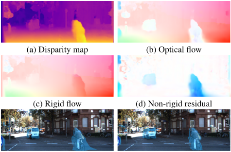
(f) Motion segmentation
Figure 1: Predictions by our method on KITTI 2015. We compared two method to segment non-rigidity (moving) region in the scene. (e) is obtained by thresholding on the non-rigid residual, and (f) is obtained by a novel method which compare the optical flow and rigid flow from the image similarity.
proposed a novel approach for unsupervised learning of both depth and ego-motion, various unsupervised methods for visual geometric estimation emerged, which using view synthesis as supervision by the underlying geometric relations [Godard et al., 2017; Meister et al., 2018].
Although unsupervised methods are able to estimate optical flow or stereo depth separately, there are still some challenges. One of the most critical issues in unsupervised geometric learning is that the correspondences in vision synthesis are ambiguous. There are more than one points in the source image that match with the same point in target image which can all minimize the photometric loss, especially in the texture-less region or area with repeating patterns. To reduce the ambiguity, a smooth regularization term like the one used in [Zhou et al., 2017] is necessary. However, the smooth regularization yields inconsistent results on the boundary of objects. Though the later works [Yin and Shi, 2018; Wang et al., 2018b] used edge-aware smooth loss, the problem still exists. In addition, there might be no point correspondence in the occlusion or non-rigid region, which affects the accuracy and stability of training. Therefore, distinguishing static areas is crucial for unsupervised geometric learning.
In this paper, we focus on scene flow estimation by decoupling into two tasks: depth and optical flow estimation. A brief example of our results is shown in Figure 1. Following the methods of unsupervised depth [Godard et al., 2017] and unsupervised optical flow [Wang et al., 2018b], we further towards exploiting the characteristics of unsupervised geometric learning and fusing with the intrinsic relationship between depth and optical flow to obtain a more accurate estimation.
More specifically, we first estimate the camera motion in a dynamic scene from the optical flow and depth predictions through an interpretable optimization method. In contrast to many prior works which assumes the pose is known [Basha et al., 2013], or estimate an initial pose followed by refinement with optimization [Lv et al., 2018], or estimated by a traditional feature-based method [Jaimez et al., 2017], our method is more concise and compact which leads to a much improved pose estimation with insignificant runtime. Then, we introduce a novel method to fuse depth and optical flow to obtain the rigidity segmentation which we represent as a binary mask with the static scene masked as rigid. Unlike other methods estimated the rigidity by thresholding on the residual of optical flow and rigid flow, which is suffering from the inconsistent in the boundary as the smooth regularization, as shown in Figure 1 (e). our method infers per-pixel rigidity by image produce a more precise segmentation, as shown in Figure 1 (f). Finally, we incorporate the rigidity mask into joint training of depth and optical flow leading a state-of-the-art performance in unsupervised scene flow estimation.
2 RelatedWork
Scene flow describes dense 3D motion in dynamic scenes. Since [Vedula et al., 1999] proposed a method to compute 3D motion fields from multi-view image sequences as a variational problem. The task of scene flow estimation has often been formulated as a single variational problem and solved using optimization methods [Valgaerts et al., 2010; Basha et al., 2013]. These methods are computationally expensive which are inappropriate for application. Recent work computing scene flow from a combination of depth and 2D optical flow have shown to be considerably faster with comparable performance. [Quiroga et al., 2014] exploits the local and piece-wise rigidity to estimate scene flow with an RGBD sensor and 6-DoF transforms. All these methods require off-the-shelf depth map with rigidity as a prior. We show that the depth and flow can be estimated from images by learning models to reconstruct the scene flow.
Learning based methods have shown the capability of estimating the necessary scene geometry for scene flow estimation. Typical supervised learning approaches have made great progress in various tasks such as stereo depth [Chang and Chen, 2018], monocular depth [Eigen et al., 2014], optical flow [Sun et al., 2018; Ilg et al., 2017], camera ego-motion estimation [Wang et al., 2018a].
While supervised learning can reach excellent performance, the ground truth is hard to acquire in real-world settings, which limits its applicability. To alleviates the difficulty of collecting data for training, an alternative solution is unsupervised learning. [Zhou et al., 2017] proposed a novel approach for learning of depth and ego-motion by selfsupervised a photometric loss on the reconstructed image by view synthesis, several unsupervised methods for visual geometric estimation have been proposed. [Godard et al., 2017] introduced a left-right consistency loss for training stereo depth from a single image. [Meister et al., 2018] first introduced an unsupervised optical flow estimation method with a bidirectional census loss, and [Wang et al., 2018b] improved the accuracy by handling the occlusions with a process similar to bilinear interpolation.
Most of the above methods rely on a rigid scene assumption, which will be corrupted by moving objects in the scene. Especially for the scene flow estimation task, it is crucial to distinguish the region in a scene into rigid and non-rigid. The framework we introduced can explicitly deal with the object motion by fusing the local rigidity with unsupervised learning. A similar strategy is used in previous works. [Jaimez et al., 2017] segment the piecewise-rigid scene by geometric clusters with an RGB-D odometry algorithm. [Wulff et al., 2017] segment scene and refine the optical flow in the static region with a plane+parallax method. [Lv et al., 2018] supervised train a network to predict the rigidity segments for scene flow estimation. However these methods unable to generalization to unsupervised learning.
Our work is inspired from some recent works in terms of unsupervised learning of scene flow and rigidity reasoning [Yin and Shi, 2018; Lee and Fowlkes, 2018; Wang et al., 2018c], but mainly differs in several ways: (1) Instead of training an additional pose network, we explicitly estimate the camera motion from the predictions of depth and optical flow through an interpretable optimization method, which is more compact for scene flow estimation. (2) We digging into the characteristics of unsupervised geometric learning and fusing with the intrinsic relationship between depth and optical flow to estimate a more accurate rigidity masks (3) The joint training framework integration with local rigidity can consistently improve the results of all subtasks.
3 Method
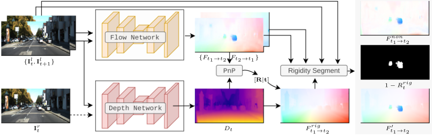
We focus on solving for the scene flow in the physical scene observed from a moving camera. Figure 2 presents an overview of our unsupervised joint learning pipeline. In the following, we will describe specific components in details.
3.1 Unsupervised Depth and Optical Flow
The key idea of most unsupervised depth or flow estimation methods are designed to implicitly minimize the differences between the reconstructed image ˆI and the original image I. The objective can be formulated by
where ρ (.) is a measure of similarity between pixels, and the image ˆI is reconstructed by view synthesis with the learnable parameters of the model Θ.
Given a source image, view synthesis uses the scene geometry to synthesize a new image in a different point of view. In terms of unsupervised optical flow, the image ˆI can be synthesized by predicted flow field Ft1→t2 . The frame ˆIt is inverse warping from the frame It+1 by
where p is the pixel coordinates. Note that the projected image coordinates are continuous values, bilinear interpolation is required for warping operation [Jaderberg et al., 2015].
In terms of unsupervised stereo depth, the network is trained to predict the disparity of a stereo image pair. The estimated disparity map can be used to synthesize one view of the stereo image pair from another view, which is similar to the optical flow scenario, except that the correspondences are horizontally aligned by the epipolar constraint. The disparity map can be converted into scaled metric depth D with known focal length and the baseline between cameras.
Supervision with view synthesis suffers from the illumination changes, correspondences ambiguity in the texture-less or homogeneous region. To handle these issue, robust similarity measurement and auxiliary regularization terms are necessary. The overall loss function and the network architecture are described in Section 3.4.
3.2 Pose Estimation fromDepth and Optical Flow
Let pt ∈ R2 be the coordinates of a pixel in the image It from a moving camera, and K denote the known camera intrinsics. Given the estimated depth Dt(pt), we can back-project pt into 3D camera coordinates by perspective project model 1 :
The corresponding 2D projection of the point xt on the image It+1 can be induced by the optical flow
Let Tt→t+1 = [R|t] ∈ R3×4 be the 6-DOF pose of the camera at time t + 1 with respect to time t in the form of its rotation and translation. The projection of the 3D point xt on the image plane of It+1 can be formulated as
1 The conversions between Homogeneous and Cartesian coordinates in this paper are omitted for notation brevity.
We know the projection of 3D points in the scene ˆpt+1 by the depth Dt, and the corresponding 2D projections pt+1 by the optical flow Ft1→t2 . The goal is to estimate the camera motion. We solve this problem by a Perspectiven-Point (PnP) with random sample consensus (RANSAC) method [Fischler and Bolles, 1981]. The objective is the sum of euclidean distances between the projection of 3D points and the image points obtained by the optical flow.
where Ω is the set of inlier correspondences in which the points should lie in the rigid region. Though segment the rigid region from a dynamic scene is a challenging task, thanks to the redundancy from dense predictions, RANSAC performs well to screen out enough inlier correspondences by a threshold δ1 of re-project distance.
Since there are a large number of 2D-3D correspondences provides this estimation with redundancy, we sample the depth and flow before the optimization. We first remove all the points with uncertain depth value follow the crop scheme in [Eigen et al., 2014]. Then we uniformly sample the correspondences with a stride of 16 in the image plane, which helps to solve the optimization more efficiently and numerically stable. We adopt the Direct Linear Transform with Levenberg-Marquardt optimization to find such a pose that minimizes the re-projection error.
3.3 Exploiting Rigidity for Joint Leaning
When a point p in a scene remains stationary, the optical flow is purely induced by the camera motion and is referred as the rigid flow
which describes the motion of a rigid scene projected onto the image plane. On the contrary, the non-rigid residual that describes the motion of the object onto the image plane can be computed by
From another perspective, the non-rigid residual is the reprojection distance mentioned in Equation (6). It can be used to obtain the rigidity region in a dynamic scene, as the value of the re-projection distance should be small in the static area and vice versa. This strategy has been used to segment the rigidity region by a threshold [Yin and Shi, 2018]. When the optical flow and rigid flow are obtained from the ground truth, it even can be used as a measurement for supervised motion segmentation task [Lv et al., 2018]. We denote the rigid region segmented by thresholding as
where [1] is an Iverson bracket, ϵ is the threshold.
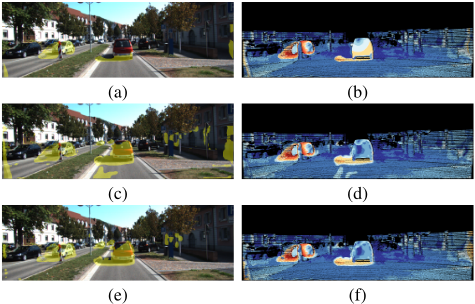
However, we argue that the predictions in the unsupervised scenario are not accurate enough to directly compute the rigidity. As demonstrated in Figure 3, optical flow around the boundary of moving objects are affected by the flow in the background due to the smooth regularization term. A larger threshold tends to miss the motion area and smaller leads to more False Positive.
We propose to estimate the rigidity region by converting flow into the image space, in which we measure the optical flow and rigid flow by inverse warping in Equation (2) to obtain the reconstructed image ˆIopt and ˆIrig respectively, and measure the pixel-wise similarity with a weighted sum between SSIM-based loss and l1 loss to form the corresponding error maps Eopt and Erig
where α is set to 0.85 and the rigidity segmentation can be
where g(.) is Gaussian blur with radius 5 to reduce the noise. We follow a basic assumption that most areas of scene are static, so δ2 is set to the 80-th percentile of Eopt .
In addition, optical flow in the occlusion area is meaningless, where the correspondence point in the next frame does not exist. We follow the occlusion estimation method proposed in [Wang et al., 2018b], which estimate the occlusion map Rocc from the backward flow, by counting the contributions of each pixel in the bilinear interpretation of inverse warp. The final local rigidity Rrig is a union of Rph and Rocc .
3.4 Network Architecture and Loss Functions
The first stage to infer scene layout is made up of two subnetworks, i.e. the flow network and the depth network. The former is based on the PWC-Net [Sun et al., 2018], a recently proposed network that achieves excellent performance in supervised learning of optical flow tasks. Especially, we replace all deconvolutional layers by bilinear upsampling.
As for the depth network, we implement both monocular and stereo networks. For the monocular scenario, we follow the structure introduced in [Godard et al., 2017], which adopt ResNet as the backbone with an encoder-decoder architecture. For the stereo scenario, we half the output channel of the flow network to predict the offset of a single channel.
The unsupervised loss in our framework is a combination of depth and optical flow. Here we briefly describe the loss functions that we used in our framework for unsupervised training.
FlowPhotometric Loss. The photometric loss is computed in the non-occlusion region only. We adopt the same measurement in Equation (10) to compute the loss
Flow Smooth Loss. In order to alleviate the effect of smooth regularization, the smooth loss is computed in the moving region only. We follow the previous works that use an edge-aware 2nd smooth loss
Stereo Depth Loss. The stereo loss Ld is the same as in [Godard et al., 2017].
Rigid Consistency Loss. In the static region, the rigid flow that considered both 3D-2D and 2D-2D correspondences is more accurate than the optical flow predictions. The rigid consistency loss to guide optical flow is formed as follow
Note that the gradient for F rig t1→t2 should be blocked.
RigidPhotometric Loss. The rigid flow is computed by the depth prediction which can accurately describe the 2D motion in the static region. The photometric loss on rigid flow can provide another point of view for depth estimation.
Final Loss. In summary, the final loss function becomes a weighted sum of the above terms at multiple scales
where λ denotes the weight for each part and i indexes the layer of output pyramid.
4 Experiments
4.1 Data
We evaluate our method on the KITTI benchmark suite. More specifically, scene flow is evaluated on the KITTI 2015 scene flow benchmark, which contains disparity, optical flow and motion segmentation. In addition, we evaluate the optical flow on the KITTI 2012 stereo flow benchmark [Geiger et al., 2012] as well, in which the camera keeps stationary [Menze and Geiger, 2015]. We adopt the images from the KITTI raw dataset [Geiger et al., 2013] for unsupervised training depth and flow models without using any ground truth of depth and optical flow. Since the KITTI raw dataset contains some samples from the validation set, we filtered all the scenes that appeared in the validation before training. Especially, Camera motion task is trained and evaluated on the KITTI odometry benchmark which is a subset of raw data.
4.2 Implementation Details
We implemented all learnable parts in PyTorch [Paszke et al., 2017]. All models are trained with the Adam optimizer [Kingma and Ba, 2015] with β1 = 0.9, β2 = 0.99, batch size of 4. We resize the images to 256 × 832 and data augmentation including random flip and time swap is used.
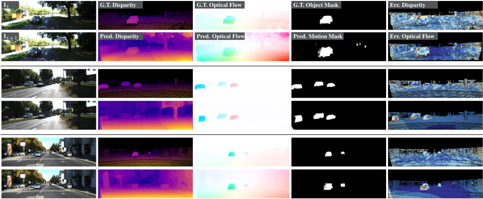
Unlike most optical flow estimation learning methods that require pre-training on multiple datasets, our approach can be trained from scratch. The training in our method contains two stages. In the first stage, we train the depth model and flow model with the loss weights λs = 80, λd = 1, λr = 0, λc = 0. The initial learning rate is 10-4 , and divided by 2 every 100k iterations, finishing at 300k iterations. In this stage, Lc and Lrig p are discarded as the rigid mask is not accurate enough to guide the training. By discarding these two losses, the optimizations of the depth model and flow are completely independent, so these two models can be trained separately. In the second stage, we fine-tune the models with the best validation accuracy in the first stage. The loss weights are change to λr = 1, λc = 0.1. The learning rate is 10-5 and finishing at 30k iterations. In addition, we train a monocular model following the setting in [Godard et al., 2017] with Resnet18 as the backbone and a stereo model with the same procedure. The visualization results of our stereo model are shown in Figure 4.
| Method | EPE Static | EPEMove | EPE All | F1 (%) |
|---|---|---|---|---|
| Separate | 6.44 | 5.08 | 6.45 | 20.44 |
| Rigid | 2.85 | 36.58 | 10.65 | 22.31 |
| Joint Training | 5.31 | 4.94 | 5.43 | 16.12 |
| Fusing with Rth | 4.57 | 8.00 | 5.77 | 15.81 |
| Fusing with Rph | 3.85 | 7.92 | 5.19 | 14.68 |
4.3 Quantitative Results
In the following, we report the results of our method on optical flow, depth, camera motion and object motion segmentation tasks.
Optical Flow
Firstly, we compare the optical flow results of several variants of our method: Separate indicates the flowmodel trained separately, i.e. the model of the first stage. Rigid indicates the rigid flow obtained by the depth and optical flow from the model in the first stage. Joint means the optical flow predictions of the model in the joint training stage. Fusing with Rth and Fusing with Rph are the results of fusing rigid flow and optical flow with Rth and Rph respectively.
The results are shown in Table 1. Rigid flow in the static region is much more precise than optical flow, and the joint training optical flow and depth models consistently improve the performance of static and moving regions. It is worth noting that the fusion rigidity with Rth can improve the accuracy of the static region, but worse in the moving region. As a compromise, fusion rigidity with Rph achieves the best comprehensive metrics EPE and F1 scores.
We also compared our method with state-of-the-art methods, including Flownet2 [Ilg et al., 2017] and PWC-Net [Sun et al., 2018] for supervised learning, UnFlow-CSS [Meister et al., 2018] for unsupervised learning, and recent works [Wang et al., 2018b; Wang et al., 2018c]. The results in Table 2 show that our method achieves the best unsupervised results on KITTI2015, in which the scene is more difficult than KITTI2012 since both cameras and scene are moving. Note that the training results of FlowNet2+ft and PWC-Net+ft are meaningless, for which are trained and validated on the same data. While on the test set, our results are very close to these supervised methods. In addition, the monocular trained model performs worse than stereo based approaches, while our fusion method still significant boost the preference.
| Setting | KITTI 2012 | KITTI 2015 | ||||||||
|---|---|---|---|---|---|---|---|---|---|---|
| Method | Train Stereo | Test Stereo | Super- vised | train Noc | train Occ | train All | train move | train static | train all | test all |
| Flownet2 | ✓ | - | - | 4.09 | - | - | 10.06 | - | ||
| Flownet2+ft | ✓ | - | - | (1.28) | - | - | (2.3) | 11.48% | ||
| PWC-Net | ✓ | - | - | 4.14 | - | - | 10.35 | - | ||
| PWC-Net+ft | ✓ | - | - | (1.45) | - | - | (2.16) | 9.60% | ||
| UnFlow-CSS | 1.26 | - | 3.29 | - | - | 8.10 | - | |||
| [Wang et al., 2018b] | - | - | 3.55 | - | - | 8.88 | 31.2% | |||
| [Wang et al., 2018c] | ✓ | ✓ | 1.04 | 5.18 | 1.64 | 5.30 | 5.39 | 5.58 | 18.00 % | |
| Ours (Monocular) | ✓ | 2.28 | 7.25 | 2.96 | 8.59 | 4.88 | 5.74 | - | ||
| Ours (Stereo) | ✓ | ✓ | 1.09 | 4.87 | 1.92 | 7.92 | 3.85 | 5.19 | 11.66% | |
| Method | Train | Test | Lower the better | Higher the better | |||||
|---|---|---|---|---|---|---|---|---|---|
| Stereo | Stereo | Abs Rel | Sq Rel | RMSE | RMSE log | δ < 1.25 | δ < 1.252 | δ < 1.253 | |
| [Zhou et al., 2017] | 0.216 | 2.255 | 7.422 | 0.299 | 0.686 | 0.873 | 0.951 | ||
| [Godard et al., 2017] | ✓ | 0.124 | 1.388 | 6.125 | 0.217 | 0.841 | 0.936 | 0.975 | |
| Ours (Monocular) | ✓ | 0.108 | 1.020 | 5.528 | 0.195 | 0.863 | 0.948 | 0.980 | |
| [Godard et al., 2017] | ✓ | ✓ | 0.068 | 0.835 | 4.392 | 0.146 | 0.942 | 0.978 | 0.989 |
| Ours (Stereo) | ✓ | ✓ | 0.051 | 0.532 | 3.780 | 0.126 | 0.957 | 0.982 | 0.991 |
Depth
The depth estimation in our method is primarily based on the work of [Godard et al., 2017], with an additional rigid photometric loss Lrig p . The results in Table 3 show that our monocular method achieving better performance, which proves the effectiveness of rigid photometric loss. However, comparing with the stereo method, the promotion is limited as the excellent performance of the original method.
Camera Motion
We evaluate the camera motion estimation on KITTI odometry benchmark, where the 00-08 sequences are used for training and the 09-10 sequences for testing. We compared our approach to the traditional SLAM method and several unsupervised methods. Since the length of the sequence used for estimation in these methods is different, we follow the metric in [Zhou et al., 2017] where the results are evaluated in terms of 5-frame trajectories. For some methods that input with less than five frames, we first compute the full trajectory and get the result for the 5-frame snippet by a sliding window. Note that although our method is capable of predicting scaled output, some methods are scale agnostic, so we still optimize the scale factor to align with the ground truth for comparison. The results in Table 4 demonstrate the effectiveness of our approach, despite the discarding of a specialized pose network.
| Method | # frames | Sequence 09 | Sequence 10 |
|---|---|---|---|
| ORB-SLAM(Full) | All | 0.014 ± 0.008 | 0.012 ± 0.011 |
| [Zhou et al., 2017] | 5 | 0.016 ± 0.009 | 0.013 ± 0.009 |
| Geonet | 5 | 0.012 ± 0.007 | 0.012 ± 0.009 |
| [Wang et al., 2018c] | 2 | 0.012 ± 0.006 | 0.012 ± 0.008 |
| Ours (Stereo) | 2 | 0.012 ± 0.007 | 0.012 ± 0.006 |
| Method | Pixel Acc. | Mean Acc. | Mean IoU | f.w. IoU |
|---|---|---|---|---|
| [Yang et al., 2018] | 0.89 | 0.75 | 0.52 | 0.87 |
| [Wang et al., 2018c] | 0.90 | 0.82 | 0.56 | 0.88 |
| Ours | 0.93 | 0.84 | 0.57 | 0.90 |
Object Motion Segmentation
We evaluate the motion segmentation task follow the setting in [Yang et al., 2018], which using the object map provided in the KITTI 2015 dataset to generate the ground truth map. As shown in Table 5, our method improvements all metrics that produce a more precise motion segmentation.
5 Conclusion
We propose a jointly unsupervised learning method of optical flow and stereo depth estimation. We demonstrate the advantages of exploiting local rigidity to fuse these two tasks. Our method reveals the capability of unsupervised learning in scene flow estimation. The impressive results compared to other baselines including the supervised methods indicate the possibility of learning scene flow without costly collected ground-truth data. For future work, we would like to find an unsupervised learning method to distinguish the rigidity region by a network in the end-to-end manner.
Acknowledgments
This work is supported in part by the National Key Research and Development Program of China under Grant 2017YFB1302003 and the National Natural Science Foundation of China under Grant U1509210.
@inproceedings{ijcai2019p123,
  title     = {Unsupervised Learning of Scene Flow Estimation Fusing with Local Rigidity},
  author    = {Liu, Liang and Zhai, Guangyao and Ye, Wenlong and Liu, Yong},
  booktitle = {Proceedings of the Twenty-Eighth International Joint Conference on
               Artificial Intelligence, {IJCAI-19}},
  publisher = {International Joint Conferences on Artificial Intelligence Organization},
  editor    = {Sarit Kraus},
  pages     = {876--882},
  year      = {2019},
  month     = {8},
  note      = {Main track},
  doi       = {10.24963/ijcai.2019/123},
  url       = {https://doi.org/10.24963/ijcai.2019/123},
}
TY - CPAPER TI - Unsupervised Learning of Scene Flow Estimation Fusing with Local Rigidity AU - Liu, Liang AU - Zhai, Guangyao AU - Ye, Wenlong AU - Liu, Yong T2 - Proceedings of the Twenty-Eighth International Joint Conference on Artificial Intelligence, IJCAI-19 PB - International Joint Conferences on Artificial Intelligence Organization PY - 2019 SP - 876 EP - 882 DO - 10.24963/ijcai.2019/123 UR - https://doi.org/10.24963/ijcai.2019/123 ER -Copied
Machine-readable versions of this paper, for tools and AI agents:





