
How to Tame Your Anticipatory Algorithm
Proceedings of the Twenty-Eighth International Joint Conference on Artificial Intelligence. Main track. Pages 1071-1077.
https://doi.org/10.24963/ijcai.2019/150
Keywords
- Heuristic Search and Game Playing: Combinatorial Search and Optimisation
- Uncertainty in AI: Uncertainty in AI
- Constraints and SAT: Constraint Satisfaction
Abstract
Sampling-based anticipatory algorithms can be very effective at solving online optimization problems under uncertainty, but their computational cost may be prohibitive in some cases. Given an arbitrary anticipatory algorithm, we present three methods that allow to retain its solution quality at a fraction of the online computational cost, via a substantial degree of offline preparation. Our approaches are obtained by combining: 1) a simple technique to identify likely future outcomes based on past observations; 2) the (expensive) offline computation of a "contingency table"; and 3) an efficient solution-fixing heuristic. We ground our techniques on two case studies: an energy management system with uncertain renewable generation and load demand, and a traveling salesman problem with uncertain travel times. In both cases, our techniques achieve high solution quality, while substantially reducing the online computation time.
- [Bai et al., 2015] Hao Bai, Shihong Miao, Xiaohong Ran, and Chang Ye. Optimal dispatch strategy of a virtual power plant containing battery switch stations in a unified electricity market. Energies, 8(3):2268-2289, 2015.
- [Bent and Van Hentenryck, 2004] Russell Bent and Pascal Van Hentenryck. Regrets only! online stochastic opti- mization under time constraints. In AAAI, volume 4, pages 501-506, 2004.
- [Bent and Van Hentenryck, 2005] Russell Bent and Pascal Van Hentenryck. Online stochastic optimization without distributions. In ICAPS, volume 5, pages 171-180, 2005.
- [Borodin and El-Yaniv, 2005] Allan Borodin and Ran El- Yaniv. Online computation and competitive analysis. cam- bridge university press, 2005.
- [Chang et al., 2000] Hyeong Soo Chang, Robert Givan, and Edwin KP Chong. On-line scheduling via sampling. In AIPS, pages 62-71, 2000.
- [De Filippo et al., 2018] Allegra De Filippo, Michele Lom- bardi, and Michela Milano. Methods for off-line/on-line optimization under uncertainty. In IJCAI, pages 1270- 1276, 2018. IJCAI
- [Dinh et al., 2016] Laurent Dinh, Jascha Sohl-Dickstein, and Samy Bengio. Density estimation using real nvp. arXiv preprint arXiv:1605.08803, 2016.
- [Espinosa and Ochoa, 2015] Alejandro N. Espinosa and Luis N. Ochoa. Dissemination document "low voltage net- works models and low carbon technology profiles". Tech- nical report, University of Manchester, June 2015.
- [Gauvain and Lee, 1994] Jean-Luc Gauvain and Chin-Hui Lee. Maximum a posteriori estimation for multivariate gaussian mixture observations of markov chains. IEEE transactions on speech and audio processing, 2(2):291- 298, 1994.
- [Hentenryck and Bent, 2009] Pascal Van Hentenryck and Russell Bent. Online stochastic combinatorial optimiza- tion. The MIT Press, 2009.
- [John and Langley, 1996] George H John and Pat Langley. Static versus dynamic sampling for data mining. In KDD, volume 96, pages 367-370, 1996.
- [Kleywegt et al., 2002] Anton J Kleywegt, Alexander Shapiro, and Tito Homem-de Mello. The sample average approximation method for stochastic discrete optimiza- tion. SIAM Journal on Optimization, 12(2):479-502, 2002.
- [Lin et al., 2013] Minlong Lin, Ke Tang, and Xin Yao. Dy- namic sampling approach to training neural networks for multiclass imbalance classification. IEEE Transactions on Neural Networks and Learning Systems, 24(4):647-660, 2013.
- [Mercier and Van Hentenryck, 2007] Luc Mercier and Pas- cal Van Hentenryck. Performance analysis of online antic- ipatory algorithms for large multistage stochastic integer programs. In IJCAI, pages 1979-1984, 2007.
- [Mercier and Van Hentenryck, 2008] Luc Mercier and Pas- cal Van Hentenryck. Amsaa: A multistep anticipatory algorithm for online stochastic combinatorial optimiza- tion. Integration of AI and OR Techniques in Constraint Programming for Combinatorial Optimization Problems, pages 173-187, 2008.
- [Palma-Behnke et al., 2011] Rodrigo Palma-Behnke, Carlos Benavides, E Aranda, Jacqueline Llanos, and Doris Sáez. Energy management system for a renewable based mi- crogrid with a demand side management mechanism. In Computational intelligence applications in smart grid (CIASG), 2011 IEEE symposium on, pages 1-8. IEEE, 2011.
- [Philpott and De Matos, 2012] Andrew B Philpott and Vi- tor L De Matos. Dynamic sampling algorithms for multi- stage stochastic programs with risk aversion. European Journal of Operational Research, 218(2):470-483, 2012.
- [Powell, 2016] Warren B. Powell. A Unified Framework for Optimization Under Uncertainty, chapter 3, pages 45-83. 2016.
- [Rezende and Mohamed, 2015] Danilo Jimenez Rezende and Shakir Mohamed. Variational inference with normalizing flows. arXiv preprint arXiv:1505.05770, 2015.
- [Sahinidis, 2004] Nikolaos V. Sahinidis. Optimization under uncertainty: state-of-the-art and opportunities. Comput- ers & Chemical Engineering, 28(6):971 -983, 2004. FO- CAPO 2003 Special issue.
- [Silverman, 2018] Bernard W Silverman. Density estimation for statistics and data analysis. Routledge, 2018.
References were extracted automatically from the PDF and may contain errors.
Full text extracted automatically from the PDF; figures, tables and equations may differ. The PDF is the version of record.
1 Introduction
Optimization problems under uncertainty arise in many important application domains, such as production scheduling or energy system management. These problems often benefit from making all or part of their decisions online, reacting and adapting to external events. In this context, stochastic online anticipatory algorithms have proved particularly effective (see e.g. [Hentenryck and Bent, 2009]). However, many of such algorithms have a considerable computational cost, which may be problematic if (as it is often the case) online decisions must be taken within a short time frame.
In most practical settings, however, a substantial amount of time and information is available before the online problem is solved, in an offline phase. For example, one may have access to energy production forecasts, historical travel times in routing problems, results from test runs in cyber-physical systems. We refer to this sort of data as offline information. Usually, it is employed to characterize the uncertain elements and for sampling likely outcomes (i.e. scenarios). We will show how to exploit this information at a much deeper level.
We propose three hybrid offline/online methods that build over a given, sampling-based, anticipatory algorithm, and allow to match its solution quality at a fraction of the online computational cost. One of them can even rely on a deterministic algorithm, thus providing state-of-the art performance in problems for which no anticipatory approach is available. All our methods work by shifting part of the computation to the offline phase, where time limits are more relaxed and the costs can be better amortized (e.g. via parallelization).
We obtain our methods by combining three basic contributions: 1) a technique to estimate the probability of future outcomes, given past observations; 2) a scheme for building a "contingency table", with precomputed solutions to guide the online choices; and 3) an efficient fixing heuristic for adapting the precomputed solutions to run-time conditions.
We ground our approaches on a (numeric) energy management problem with uncertain loads and generation from Renewable Energy Sources (RES), and on a (discrete) Traveling Salesman Problem with uncertain travel times. We show how our methods reach a solution quality comparable with the anticipatory algorithm, with lower (or dramatically lower) online computational cost.
The paper is structured as follows: in Section 2 we cover background and related works. We show our contributions in Section 3 and their grounding in Section 4. Experimental results are in Section 5 and concluding remarks in Section 6.
2 Background and RelatedWork
Historically, the literature on optimization under uncertainty has focused on offline problems [Powell, 2016; Sahinidis, 2004]. These methods usually rely on sampling (yielding a number of scenarios) to obtain a statistical model of future uncertainty. Robust solutions can be obtained by building one copy of the decision variables per scenario, and linking them via non-anticipativity constraints (decisions based on the same observations should be identical). This is known as the Sample Average Approximation method [Kleywegt et al., 2002]: it provides convergence guarantees under reasonable assumptions, and can substantially outperform myopic optimization.
More recently, improvements in the solution techniques and computational power have enabled the application of similar methods to online optimization. This lead to so-called online anticipatory algorithms, which proved very effective at finding robust, high quality, solutions as uncertainty slowly reveals itself. A very good overview of this line of research is provided by [Hentenryck and Bent, 2009], while notable algorithms and results are described in [Chang et al., 2000; Bent and Van Hentenryck, 2004; 2005; Mercier and Van Hentenryck, 2008; De Filippo et al., 2018].
Online anticipatory algorithm typically rely on scenario sampling to estimate the possible developments for a fixed number of future steps, known as look-ahead horizon. Larger sample sizes result in higher accuracy, but also in more and bigger (possibly NP-hard) problems to be solved. This is a strong limitation, since in many practical cases online decision must be produced within strict time limits. Considerable research effort has therefore focused on improving the efficiency of these algorithms. For example, the CONSENSUS and REGRET algorithms from [Bent and Van Hentenryck, 2004] both attempt to reduce the number of problems w.r.t. the earlier EXPECTATION approach. Computational studies such as [Borodin and El-Yaniv, 2005; Mercier and Van Hentenryck, 2007] aim at characterizing the algorithm sensitivities to their design parameters (such as the number of sampled scenarios and the look-ahead horizon). The approaches from [John and Langley, 1996; Philpott and De Matos, 2012; Lin et al., 2013] attempt instead to reduce the number of scenarios by increasing their relevance, and in particular by taking into account past observations while sampling.
3 "Taming" an Anticipatory Algorithm
Our goal is reducing the online computational cost of a given sampling-based anticipatory algorithm, referred to as A, by exploiting the existence of an offline phase. Such A algorithm is the main input for all our methods.
Similarly to [Hentenryck and Bent, 2009], we view online optimization under uncertainty as a stochastic n-stage problem. At each stage some uncertainty is resolved, and some decision must be made. A stage k is associated to a decision variable xk (e.g. the power flows between loads and generators) and a state variable sk (summarizing the effect of past decisions). All variables may be vector-valued.
We assume that uncertainty is exogenous, i.e. not affected by the decisions (e.g. the RES generation does not depend on how we choose to route it), and modeled via a set of random variables ξi. Which variables are observed at each stage depends on the state, and is controlled by a peek function:
which returns a set O with the indices of the observed variables. We will use the notation ξO to denote the observed ξ variables, and ξ ¯O for the unobserved ones.
Base Anticipatory Algorithm
Sampling-based algorithms rely on scenarios to estimate future outcomes. Formally, a scenario ω specifies a value ξω i for all the random variables. Given a set Ω of scenarios, the system state sk, and values for ξO corresponding to the observed uncertainty, we assume that A can compute the decisions for stage k:
Once the decisions are computed, the next state can be determined. This is controlled via a state transition function next
Algorithm 1 ANTICIPATE (s1, ξ)
| Sample a set of scenarios Ω for k = 1 . . . n do O = O ∪ peek(sk) xk = A(sk, ξO, {ξω }ω∈Ω) sk+1 = next(sk, xk, ξO) return s, x | # observe uncertainty # obtain decisions # determine next state |
that, based on the current state, decisions, and observed uncertainty, computes:
Given the initial state s1, a set of scenarios Ω, and a set of values sampled from ξk (which represent the online observations), we can simulate the execution of the method via Algorithm 1. The O set is assumed to be initially empty. This generic anticipatory algorithm will be referred to as ANTICIPATE in the remainder of the paper.
Offline Information
Defining a representative set of scenarios Ω is critical for the approach effectiveness and it is usually done by exploiting the available offline information. Here, we assume that the such offline information is a collection of observed uncertain values. This definition captures many practical cases (e.g. forecasts or predictions, historical data, data from test runs). More importantly, this means that the offline information is in fact a collection of scenarios. We will denote the offline information as I, index its element with ω, and assume (as it is usual) that I is representative of the true probability distribution of the random variables. A set Ω of scenarios for ANTICIPATE can be obtained by sampling a number of elements uniformly at random from I.
3.1 Basic Contributions
All our methods rely on three techniques, which will be described in this section.
Probability Estimation for Scenario Sampling
Using a fixed set of scenarios (as in ANTICIPATE) is beneficial when the ξi variables are statistically independent. When they are not, however, the set of scenarios may loose relevance as uncertainty is resolved. For example, a scenario based on a cloudy day forecast becomes less likely if fair weather is observed at the beginning of online execution.
Formally, at stage k we wish to sample scenarios that are likely to occur given the past observations, i.e. to sample the unobserved variables ξ ¯O according to the conditional distribution P(ξ ¯O | ξO). If we draw the scenarios from the offline information (which guarantees physically meaningfulness), then sampling requires to estimate the conditional probabilities of the elements in I. From basic probability theory, this is given by the ratio of two joint probabilities:
where P(ξOξω¯O ) is the probability that observed values occur together with the remaining predictions from the scenario, and P (ξO) is the probability that the values are observed. The
Algorithm 2 BUILDTABLE (s1, AA)
joint probability at the numerator can be approximated via any density estimation method, such as Kernel Density Estimation [Silverman, 2018], Gaussian Mixture Models [Gauvain and Lee, 1994], or recent Deep Learning techniques such as Normalizing Flows [Rezende and Mohamed, 2015] and Real NVP [Dinh et al., 2016]. Any such method can be trained on the offline information to obtain an estimator ˜ P (ξ) for the joint distribution of the random variables.
An estimator for the distribution P(ξO) at the denominator can then be derived from ˜ P(ξ) via marginalization, i.e. by averaging the contribution of the unobserved variables. We perform this step over all possible completions of the observed values in the offline information. Overall, we have:
This estimator defines a discrete distribution over the offline information I. The chosen marginalization technique guarantees an estimate that is approximately proportional (not approximately equal) to the true P(ξO). Hence, we have that:
Sampling from I according to Equation (5) yields scenarios with a distribution that takes into account the observed values.
Building a Contingency Table
If a significant amount of time is available in the offline phase, we can exploit the offline information more aggressively, by trying to prepare for each likely future development. Intuitively, we can treat each scenario ω ∈ I as if it were an actual sequence of online observations, and process it via some anticipatory algorithm. By doing this, we build a pool of solutions that can then be used to guide an online method.
The process is outlined in Algorithm 2, which requires as input the initial state s1 of the system, and a solution algorithm AA, accepting the same parameters as ANTICIPATE. The result is an augmented version of the offline information, where each scenario ω is additionally associated to the sequence of states sω visited by the algorithm and its sequence of decisions xω . We refer to this data structure as contingency table, and to its elements as traces. We denote the table as T .
Fixing Heuristic
We use the traces from T to guide an efficient fixing heuristic, which tries to choose decisions having the largest chance of being optimal. Formally, it solves:
where P ∗ is the probability that the chosen xk is optimal, given the state sk and the observed uncertainty. The Xk set represents the feasible decision space, which is defined via problem-dependent constraints and auxiliary variables.
Algorithm 3 FIXING (s1, ξ, T)
Ω = top elements in T by descending Equation (10)
for k = 1 . . . n do O = O ∪ peek(sk) Compute pjv and/or pω based on Ω Solve Equation (8)/(11) to obtain xk sk+1 = next(sk, xk, ξO) return s, xClosed-forms for P ∗ can be obtained separately for discrete and numeric problems, based on the contingency table. The process is described in detail in Appendix A, and relies on several approximations. Overall, in case of discrete decisions, the problem from Equation (7) translates into:
where J·K denotes the truth value of a predicate, Dj is the domain of xkj , and:
Here, P(ω) is a compact notation for the probability that we reach the same state as trace ω, and then everything goes according to plan. It can be approximated using:
where ˜ P(ξ ¯O | ξO) is the estimator from Equation (5), and ˜ P(ssk+1 | sk) is a second estimator obtained via similar means. The cost function in Equation (8) is linear if a one-hot encoding is adopted for xkj , and the size of T affects only the computation of the pjv values. Overall, the problem is efficient to solve. In case of numeric decisions, we have instead:
with:
The cost function is quadratic and convex, and the problem size is small due to the same arguments as Equation (8).
Intuitively, the discrete version of the heuristic is related to minimizing weighted discrepancies w.r.t. the traces in T, i.e. to weighted Hamming distances. The numeric version is instead related to weighted Euclidean distances. The pseudocode for the heuristic is provided in Algorithm 3. The only difference with the process described so far is that the pjv and pω probabilities may be computed based on a subset Ω of the full contingency table. This may be useful to bias the choice of the online decision according to the most relevant traces.
3.2 Hybrid Offline/Online Methods
Our three solution methods can now be defined with relative ease, by combining the techniques just described.
Algorithm 4 ANTICIPATE-D (s1, ξ)
Train the ˜ P(ξ) estimator on I
for k = 1 . . . n do O = O ∪ peek(sk) Sample Ω from T , according to Equation (5) xk = A(sk, ξO, {ξω }ω∈Ω) sk+1 = next(sk, xk, ξO) return s, xAlgorithm 5 CONTINGENCY (s1, ξ)
Train the ˜ P(ξ) estimator on I T = BUILDTABLE(s1, ANTICIPATE) Train the ˜ P(sksk+1) estimators on T , for all k s, x = FIXING(s1, ξ, T )
return s, x
ANTICIPATE-D. Our first hybrid method is obtained from ANTICIPATE by simply replacing the static set of samples with a dynamically adjusted one. The dynamic set can be populated according to the estimated probabilities from Equation (5), so as not to loose relevance: this may enable to reach similar solution qualities with fewer scenarios, at the cost of training an estimator offline. We refer to this approach as ANTICIPATE-D, and its pseudo-code is in Algorithm 4
CONTINGENCY. The second method is based on the idea of computing robust solutions for the scenarios in the offline information, and then use them as guidance for the FIXING heuristic. Robust solutions are obtained by using ANTICIPATE, so that hopefully the (fast) fixing heuristic will be able to match their quality: the price to pay is a hefty offline computational effort. We refer to this approach as CONTINGENCY, and its pseudo-code is reported in Algorithm 5.
CONTINGENCY-D. Our final method is similar to the previous one, except that the contingency table is populated with non-robust solutions. This is done by using ANTICIPATE with a single scenario, given by the values of ξω (i.e. the pretend online observations). This technique (referred to as ANTICIPATE1) provides perfect information about the future, so that achieving robustness is entirely delegated to the FIXING heuristic. The approach is likely to loose reliability, but has two important advantages: 1) lower offline computational costs; and 2) while ANTICIPATE is a stochastic algorithm, ANTICIPATE1 is deterministic. So, this method may provide anticipatory-like results even when no anticipatory algorithm is available. We refer to this method as CONTINGENCY-D, and its pseudo-code is reported in Algorithm 6.
4 Grounding the Approaches
Grounding our approaches requires to specify: 1) the x, s and ξ variables, 2) the peek and next functions, 3) the samplingbased algorithmA, and 4) the feasible space Xk for the FIXING heuristic. Additionally, evaluating the solution quality requires to define 5) a cost metric.
We show how this can be done in two case studies: 1) a Virtual Power Plant energy management problem with numerical
Algorithm 6 CONTINGENCY-D (s1, ξ)
Train the ˜ P(ξ) estimator on I T = BUILDTABLE(s1, ANTICIPATE1) Train the ˜ P(sksk+1) estimators on T , for all k s, x = FIXING(s1, ξ, T ) return s, xdecisions; and 2) a combinatorial Traveling Salesman Problem with uncertain travel times. In both cases, the input anticipatory algorithm A is given by a Mathematical Programming model, based on the Sample Average Approximation. The models are slight improvements over those by [De Filippo et al., 2018], whose work brought to attention the interplay between offline and online phases. Both approaches are serviceable, but not necessarily representative of the state-ofthe-art (especially for the TSP). The full useful information for grounding our approaches are in a companion repository 1 , while here we focus on the minimal information needed.
4.1 The VPP Case Study.
A Virtual Power Plant aggregates different sources of power generation and consumption to offer a predictable power envelope. Managing a VPP requires to route power flows so as to satisfy the demand, to obey physical limits, and to minimize the operating costs [Palma-Behnke et al., 2011; Bai et al., 2015]. Both the demand and the RES generation are uncertain. Formally, the decision vector xk specifies the power flow xkj to/from each node (demand, generator, storage. . . ). In particular, we assume that xkS refers to flow for the storage system. The state component skS corresponds to the storage charge level, while skD to its flow direction. The random variable ξkL corresponds to the load, while ξkR to the RES generation. The peek function simply returns the pairs (k, L) and (k, R). The next function is given by:
where η is the charging efficiency of the storage system. The feasible space Xk is given by the Mathematical Program:
where Eq. (15) enforces power balance, Eq. (16) states the physical limits for the power flows, and Eq. (17) those for the storage charge. The cost incurred at each stage is given by:
where ckj is a cost associate to each flow. Unlike the model from [De Filippo et al., 2018], we include a cost term α related to storage wear-off, which increases each time the corresponding flow switches direction. Due to this term, the input algorithm A needs to solve an NP-hard problem, while the fixing heuristic has no such need.
1 https://github.com/alleDe/OffOn
4.2 The TSP Case Study.
As a second case study, we consider a TSP over an asymmetric, fully connected, graph with uncertain, exogenous, travel times (e.g. the visits have a negligible impact on traffic). In this case, the xk vector includes m components xkj, each equal to 1 iff j is the next node to be visited. There is no xkj variable for the depot, which is reached by default once all other nodes are visited. The state vector contains a component skj equal to 1 iff node j (excluding the depot) has been visited at stage k, plus a skC component specifying the index of the current node. The uncertainty is modeled via random variables ξij , each associated to the travel time between nodes i and j. The travel times for all outgoing arcs from i are observed when the node is visited, i.e. the peek function returns the pairs (skC, j) with j ∈ [1..m]. The next function is:
where Equation (20) makes sure that the value sk+1,C matches the index of the next node to be visited. The feasible space Xk is given by the Mathematical Program:
which forces moving to a single, unvisited node. The cost incurred at each stage is the travel time to the next node, i.e.:
The final cost is obtained by summing the cost of each stage, plus the distance from the last visited node to the depot. Once again, while the anticipatory algorithm A needs to solve an NP-hard problem (stochastic TSP), the fixing heuristic has no such need and is therefore much faster.
5 Experimentation
We empirically evaluated the three hybrid offline/online methods on realistic instances for the two case studies. The baseline in both cases are myopic heuristics, obtained by running ANTICIPATE with an empty set of scenarios.
5.1 Experimental Setup
Our methods are evaluated over different uncertainty realizations, obtained by sampling the random variables for the loads and RES generation in the VPP, and for the travel times in the TSP. We use models of uncertainty that ensure realistic statistical dependence between the variables. This process yields the offline information I and the sequences of observations for the experiments.
For the VPP, grid electricity prices change every 15 minutes, which is also the duration of our online stages. New offline information (e.g. market prices) becomes available every day, hence our horizon corresponds to 24 × 4 = 96 stages. We use (real) physical bounds for power generation from [Bai et al., 2015; Espinosa and Ochoa, 2015]. The initial battery state, efficiency, and power flow limit, etc. are also based on real data [Bai et al., 2015; Espinosa and Ochoa, 2015]. Different instances have then been obtained by manually scaling load and RES generation. For the TSP we use classical benchmarks 2 , by including problems from 10 to 40 nodes. In the TSP each stage represents a visit, hence our horizon corresponds to the total number of nodes.
We use Kernel Density Estimation (with Gaussian Kernels) to obtain all approximate distributions. As an underlying solver we use Gurobi 3 , which can handle both MILPs and Quadratic Programs. Each evaluated algorithm and configuration is run 50 times, with the same 50 sequences of realizations. We use a time limit of 300 seconds for both the VPP and the TSP. For each run we record both the time required by each approach and the corresponding solution cost, and we report their average values over the 50 realizations. In all cases, |I| = |T| = 100, and for the CONTINGENCY method, the contingency table is built using ANTICIPATE with 20 scenarios. Due to space constraints, we report results only for a few representative instances.
5.2 Discussion
The offline training times of the KDE models are roughly the same for all the three hybrid methods (∼ 65 sec for the VPP and ∼ 32 sec for the TSP). Building the contingency tables for CONTINGENCY takes ∼ 6, 000 sec in the VPP and ∼ 15, 000 sec in the TSP, but only ∼ 400 and ∼ 2, 000 sec for CONTINGENCY-D.
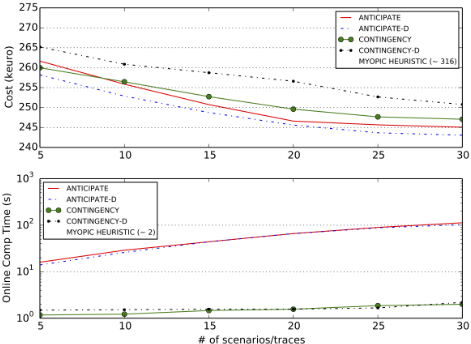
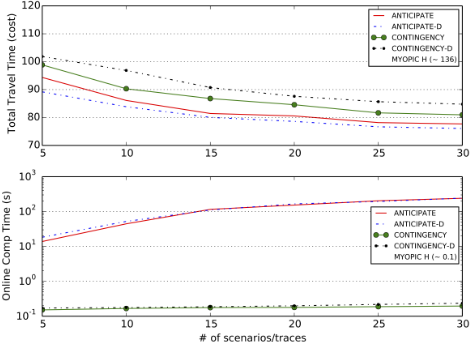
In Figure 1 we show the cost/quality tradeoff of the proposed methods and of ANTICIPATE for the VPP (base instance) and in Figure 2 for the TSP (a representative 20 customers instance). The use of a dynamic set of scenarios allows ANTICIPATE-D to work better than ANTICIPATE. The CONTINGENCY method is surprisingly close in terms of quality to the original anticipatory algorithm, especially considered its dramatically smaller online computational cost (up to two orders of magnitude). CONTINGENCY-D performs slightly worse than CONTINGENCY, but it still much better than the myopic heuristic. Increasing the number of guiding traces is beneficial in particular for CONTINGENCY-D.
2 http://myweb.uiowa.edu/bthoa/TSPTWBenchmarkDataSets.htm
3 Available at http://www.gurobi.com
| Method | VPP (σ) | TSP (σ) |
|---|---|---|
| Myopic H | 8.499 | 7.106 |
| ANTICIPATE | 4.994 | 1.889 |
| ANTICIPATE-D | 5.730 | 2.846 |
| CONTINGENCY | 5.557 | 3.788 |
| CONTINGENCY-D | 7.017 | 5.934 |
In Table 1 we show the standard deviation for the solution quality over the 50 realizations with 20 scenarios/traces for both the VPP and the TSP (on the same instances as Figure 1 and Figure 2). All values are significantly lower than the quality gap with the myopic heuristic. As expected CONTINGENCY-D tends to be less stable than the other methods due to its reliance on non-robust guiding traces.
6 Conclusion
We have presented three methods that can be applied to a generic anticipatory algorithm to reduce its online computational effort by exploiting offline information. In particular, both CONTINGENCY and CONTINGENCY-D are dramatically faster than ANTICIPATE during online operation; CONTINGENCY is significantly more reliable in terms of quality, but may require a substantial amount of offline computation. The ANTICIPATE-D technique provides a modest advantage in terms of solution time, but can match and even surpass ANTICIPATE in terms of quality.
The ability to shift part of the computational cost to an offline stage provides a significant degree of flexibility to stochastic anticipatory algorithms, and is likely to increase their applicability. We believe there is room for improving the scalability and efficiency of our methods, and achieving this goal is part of our current research directions. We also plan to apply our approaches to different application problems.
Acknowledgments
This work has been partially supported by the H2020 Project AI4EU (g.a. 825619), the VIRTUS Project (CCSEB-00094) and the Emilia-Romagna Region.
A Deriving the FIXING Heuristic
Our main goal will be to obtain a closed-form for P ∗ in Equation (7), which will require several approximations. We start by treating all components in xk as statistically independent. This allows to state P ∗ as a product of P ∗ (xkj | skξO) probabilities, related to individual components of xk. Applying a log transformation then leads to the equivalent problem:
where m is the cardinality of xk. We then assume that a decision xkj is optimal if the current optimization process is similar to a trace in the contingency table, and xkj is similar to the decision made in that circumstance. Formally, we can obtain P ∗ (xkj ) via marginalization:
where P(ω) is compact notation for P(sωk+1 ξω¯O | ξOsk). By assuming independence between the s and ξ variables, and applying the techniques used for Equation (5), we get:
where the estimator for ˜ P(sksk+1) can be trained over data from the contingency table. We now need a way to estimate P ∗ (xkj | ω). In the discrete case, we assume that xkj is optimal iff it matches the value from the contingency table, i.e. P ∗ (xkj | ω) is equal to the truth value of the predicate xki = xωkj . Hence, Equation (26) becomes:
with pjv as in Equation (9). By applying the log transformation, and using the fact that values in Dj are mutually exclusive, we get the discrete formulation from Equation (8).
In the numeric case, we assume that decisions close to the one in the trace have a chance of being optimal, which follows a Normal distribution. Formally, we have that:
where σj is the standard deviation of the value of xkj in the contingency table. By applying the log transformation to Equation (26), then Jensen's inequality, and by getting rid of offset terms (which have no impact on optimization), we get the numeric formulation from Equation (11). Note that, due to the use of Jensen's inequality, the resulting cost function is actually an approximated upper bound for the original probability.
@inproceedings{ijcai2019p150,
  title     = {How to Tame Your Anticipatory Algorithm},
  author    = {De Filippo, Allegra and Lombardi, Michele and Milano, Michela},
  booktitle = {Proceedings of the Twenty-Eighth International Joint Conference on
               Artificial Intelligence, {IJCAI-19}},
  publisher = {International Joint Conferences on Artificial Intelligence Organization},
  editor    = {Sarit Kraus},
  pages     = {1071--1077},
  year      = {2019},
  month     = {8},
  note      = {Main track},
  doi       = {10.24963/ijcai.2019/150},
  url       = {https://doi.org/10.24963/ijcai.2019/150},
}
TY - CPAPER TI - How to Tame Your Anticipatory Algorithm AU - De Filippo, Allegra AU - Lombardi, Michele AU - Milano, Michela T2 - Proceedings of the Twenty-Eighth International Joint Conference on Artificial Intelligence, IJCAI-19 PB - International Joint Conferences on Artificial Intelligence Organization PY - 2019 SP - 1071 EP - 1077 DO - 10.24963/ijcai.2019/150 UR - https://doi.org/10.24963/ijcai.2019/150 ER -Copied
Machine-readable versions of this paper, for tools and AI agents:





