
Confirmatory Bayesian Online Change Point Detection in the Covariance Structure of Gaussian Processes
Proceedings of the Twenty-Eighth International Joint Conference on Artificial Intelligence. Main track. Pages 2449-2455.
https://doi.org/10.24963/ijcai.2019/340
Keywords
- Machine Learning: Probabilistic Machine Learning
- Uncertainty in AI: Uncertainty in AI
- Machine Learning: Time-series;Data Streams
Abstract
In the analysis of sequential data, the detection of abrupt changes is important in predicting future events. In this paper, we propose statistical hypothesis tests for detecting covariance structure changes in locally smooth time series modeled by Gaussian Processes (GPs). We provide theoretically justified thresholds for the tests, and use them to improve Bayesian Online Change Point Detection (BOCPD) by confirming statistically significant changes and non-changes. Our Confirmatory BOCPD (CBOCPD) algorithm finds multiple structural breaks in GPs even when hyperparameters are not tuned precisely. We also provide conditions under which CBOCPD provides the lower prediction error compared to BOCPD. Experimental results on synthetic and real-world datasets show that our proposed algorithm outperforms existing methods for the prediction of nonstationarity in terms of both regression error and log-likelihood.
- [Adams and MacKay, 2007] Ryan Prescott Adams and David J.C. MacKay. Bayesian online changepoint detection. arXiv preprint arXiv:0710.3742, 2007.
- [Balek, 1977] Jaroslav Balek. Hydrology and Water Re- sources in Tropical Africa. Developments in water science. Elsevier Scientific Publishing Company, 1977.
- [Barry and Hartigan, 1993] Daniel Barry and John A. Harti- gan. A bayesian analysis for change point problems. Jour- nal of the American Statistical Association, pages 309-319, 1993.
- [Chernoff and Zacks, 1964] Herman Chernoff and Shele- myahu Zacks. Estimating the current mean of a normal distribution which is subjected to changes in time. The Annals of Mathematical Statistics, pages 999-1018, 1964.
- [Chow, 1960] Gregory C. Chow. Tests of equality between sets of coefficients in two linear regressions. Econometrica, pages 591-605, 1960.
- [Cleland et al., 2014] Ian Cleland, Manhyung Han, Chris Nu- gent, Hosung Lee, Sally McClean, Shuai Zhang, and Sungy- oung Lee. Evaluation of prompted annotation of activity data recorded from a smart phone. Sensors, pages 15861- 15879, 2014.
- [Eric et al., 2008] Moulines Eric, Francis R. Bach, and Zaïd Harchaoui. Testing for homogeneity with kernel fisher discriminant analysis. In Proceedings of the Neural Infor- mation Processing Systems, pages 609-616, 2008.
- [Ewing and Malik, 2016] Bradley T. Ewing and Farooq Ma- lik. Volatility spillovers between oil prices and the stock market under structural breaks. Global Finance Journal, pages 12-23, 2016.
- [Garnett et al., 2010] Roman Garnett, Michael A. Osborne, Steven Reece, Alex Rogers, and Stephen J. Roberts. Se- quential bayesian prediction in the presence of change- points and faults. The Computer Journal, pages 1430-1446, 2010.
- [Gombay et al., 1996] Edit Gombay, Lajos Horváth, and Marie Husková. Estimators and tests for change in vari- ances. Statistics and Risk Modeling, pages 145-160, 1996.
- [Gretton et al., 2012] Arthur Gretton, Karsten M. Borgwardt, Malte J. Rasch, Bernhard Schölkopf, and Alexander Smola. A kernel two-sample test. Journal of Machine Learning Research, pages 723-773, 2012.
- [Isupova, 2017] Olga Isupova. Machine learning methods for behaviour analysis and anomaly detection in video. PhD thesis, University of Sheffield, 2017.
- [Keshavarz et al., 2018] Hossein Keshavarz, Clayton Scott, and XuanLong Nguyen. Optimal change point detection in gaussian processes. Journal of Statistical Planning and Inference, pages 151-178, 2018.
- [Kim and Choi, 2015] Taehoon Kim and Jaesik Choi. Read- ing documents for bayesian online change point detection. In Proceedings of the Empirical Methods in Natural Lan- guage Processing, pages 1610-1619, 2015.
- [Kim et al., 2009] Seung-Jean Kim, Kwangmoo Koh, Stephen Boyd, and Dimitry Gorinevsky. l 1 trend filtering. SIAM review, pages 339-360, 2009.
- [Li et al., 2015] Shuang Li, Yao Xie, Hanjun Dai, and Le Song. M-statistic for kernel change-point detection. In Proceedings of the Neural Information Processing Systems, pages 3366-3374, 2015.
- [Manogaran and Lopez, 2018] Gunasekaran Manogaran and Daphne Lopez. Spatial cumulative sum algorithm with big data analytics for climate change detection. Computers and Electrical Engineering, pages 207-221, 2018.
- [Panda and Nayak, 2016] Soumya Priyadarsini Panda and Ajit Kumar Nayak. Automatic speech segmentation in syllable centric speech recognition system. International Journal of Speech Technology, pages 9-18, 2016.
- [Popper, 1951] William Popper. The Cairo Nilometer: Stud- ies in Ibn Taghrî Birdî's Chronicles of Egypt: I. Publica- tions in Semitic Philology. University of California Press, 1951.
- [Saatc ¸i et al., 2010] Yunus Saatc ¸i, Ryan D. Turner, and Carl E. Rasmussen. Gaussian process change point models. In Proceedings of the International Conference on Machine Learning, pages 927-934, 2010.
- [Sugiyama et al., 2008] Masashi Sugiyama, Taiji Suzuki, Shinichi Nakajima, Hisashi Kashima, Paul von Bünau, and Motoaki Kawanabe. Direct importance estimation for co- variate shift adaptation. Annals of the Institute of Statistical Mathematics, pages 699-746, 2008.
- [Tewkesbury et al., 2015] Andrew P. Tewkesbury, Alexis J. Comber, Nicholas J. Tate, Alistair Lamb, and Peter F. Fisher. A critical synthesis of remotely sensed optical image change detection techniques. Remote Sensing of Environment, pages 1-14, 2015.
- [Xuan and Murphy, 2007] Xiang Xuan and Kevin Murphy. Modeling changing dependency structure in multivariate time series. In Proceedings of the International Conference on Machine Learning, pages 1055-1062, 2007.
References were extracted automatically from the PDF and may contain errors.
Full text extracted automatically from the PDF; figures, tables and equations may differ. The PDF is the version of record.
1 Introduction
In sequential data, the change point detection (CPD) problem, i.e., analysis of the data with the aim of detecting abrupt changes, is an important component in improving the prediction of future events. When the underlying distribution does not change (stationary), predicting future events becomes tractable. However, the stationarity assumption does not hold in practice.
A change point (CP) is a specific sequential position at which the underlying distribution changes. CPs play critical roles in numerous real-world applications, including climate modeling [Manogaran and Lopez, 2018], speech recognition [Panda and Nayak, 2016], image analysis [Tewkesbury et al., 2015], and human activity recognition [Cleland et al., 2014]. In econometrics, structural breaks, which essentially apply CPD to regression models, have been studied for decades in an attempt to identify structural stability in forecasting time series [Chow, 1960; Ewing and Malik, 2016]. Trend filtering determines CPs by assuming piecewise linearity in the sequential data [Kim et al., 2009]. CPD also plays an important role in the domain adaptation problem known as a covariate shift [Sugiyama et al., 2008], as the distribution of the test data changes from that of the training data.
∗Equally contributed
†Contact Author
Most existing CPD methods are based on either statistical (Bayesian) inference or hypothesis tests. Statistical inference methods compute the probability of the occurrence of a change. Bayesian CPD algorithms [Barry and Hartigan, 1993; Xuan and Murphy, 2007] identify CPs using Bayesian framework. BOCPD algorithms [Adams and MacKay, 2007; Garnett et al., 2010; Saatc¸i et al., 2010; Kim and Choi, 2015] detect CPs sequentially considering the correlated interval, the so-called run length, between CPs. Such probabilistic methods, however, do not provide a statistical error bound leading to a lack of reliability and are highly sensitive to selected hyperparameters.
Hypothesis-test-based approaches determine the existence of changes based on a statistical test, where the error probability is naturally determined during the computation. Representative hypothesis test techniques include kernel methods such as two-sample tests based on the maximum mean discrepancy [Gretton et al., 2012; Li et al., 2015], kernel Fisher discriminant ratio [Eric et al., 2008], and likelihood ratio tests (LRTs) such as the cumulative sum (CUSUM) test [Chernoff and Zacks, 1964; Gombay et al., 1996]. While the conventional GPs only deal with stationary (globally smooth) functions, GPs with CPs can mimic locally smooth functions [Saatc¸i et al., 2010], allowing them to represent many real-world time series data. There have been a number of studies of CPD in GPs using hypothesis tests. For instance, CPD in GPs using p-value test on the likelihood given the null hypothesis of stationary time series has been investigated [Isupova, 2017]. If the null distribution is not legitimate, this approach cannot decisively say there is a change even if the null hypothesis is rejected. Another work has studied to detect the mean changes in GPs through LRTs [Keshavarz et al., 2018].
In this paper, we propose new statistical LRTs that detect changes in the covariance structure of GPs and build a theoretically justified online detection algorithm, Confirmatory BOCPD, which detects CPs with a reasonable time delay. We also present sufficient conditions under which CBOCPD provides the lower prediction error compared to BOCPD. Moreover, our algorithm adjusts the parameter of BOCPD to avoid false alarms and missed detections when the results of hy-
-2
0
5
10
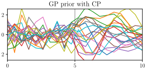
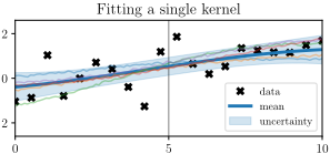
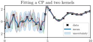
Figure 1: Left: GP prior with a covariance structure change. Middle: GP posterior after fitting data with a single kernel. Right: GP posterior after fitting data with two kernels with a CP.
pothesis tests are sound. When the results are not sound, our algorithm takes advantages of Bayesian inference from BOCPD.
2 Background
2.1 GPModels and Assumptions
A GP is a random process produced by a collection of random variables such that any finite set of those variables follows a multivariate Gaussian distribution. A GP is completely specified by the mean function µ(·) = E[f(·)] and the kernel function K(·, ·) = Cov(f(·), f(·)). The kernel function describes distinctive characteristics of the sequential data, such as variance, length scales, and periodicity. For example, in the case of the Radial Basis Function kernel K(t, t′ ) = σ2 exp(- (t-t′ )2 2l2 ), the length scale hyperparameter l controls the smoothness of the sequential data.
In this paper, we assume that observations are corrupted by the white Gaussian noise with the variance σ2no . In modeling sequential data using GPs, the index t is considered as the input, and the corresponding output is modeled as xt ∼ N(f(t), σ2no ). Given the GP hyperparameters θm and σno, the log marginal likelihood of the GP over the observed samples x is specified by the mean vector µ and the covariance matrix Σ for the multivariate Gaussian distribution. 1
2.2 Optimal CPD of the Mean
Here, we briefly review some results on the detection of a single CP in the mean function of a GP [Keshavarz et al., 2018]. The goal is to set a formal statistical test that can identify a change in the mean function and to quantify the confidence of a change.
We denote the n observed sequential data as X = {Xt }n t=1 . Let t ∈ Cn ⊆ {1, ..., n} represents the point at which a sudden change occurs. Given sequential points, two hypotheses are used for the LRT. One is the null hypothesis, H0, which insists there is no CP. The other is the alternative hypothesis, H1, which declares there is at least one CP. The hypothesis testing problem is constructed as follows. Given the two hypotheses, the likelihood ratio (LR) is defined as 2L = 2(supθ∈Θ1 ℓ(θ1)- supθ∈Θ0 ℓ(θ0)) where ℓ is the log-likelihood function and Θ0 and Θ1 are the parameter spaces of H0 and H1 respectively.
The generalized likelihood ratio test (GLRT) is formulated as TGLRT = I (2L ≥ Rn,δ) with a proper threshold Rn,δ and the indicator function I(·). Here, δ is the upper bound of the corresponding conditional detection error probability ϕn(T), which is defined as
1 log p(x|θm, σno) = - 12 (x-µ)T (Σ + σ2noI)-1 (x-µ) - 12 log |Σ + σ2noI| - n2 log 2π, where n is the number of observed samples.
We reject H0 when TGLRT=1, and we fail to reject H0, otherwise. In the mean change detection problem in a GP, we assume that the samples are generated by a GP with zero mean under the null hypothesis, which can be stated as H0 : EX = 0. Under the associative alternative hypothesis at time t, we assume that there is a change of size b in the mean as H1,t : ∃ b ̸= 0, EX = b2 ζt, where ζt ∈ Rn is given by ζt(k) := sign(k - t) for any t ∈ Cn. Combining all possible cases, the alternative hypothesis can be written as H1 : ⋃t∈Cn H1,t, which states that there exists at least one CP with jump size b. Further, we can write 2L as
where Σ is the covariance matrix of X. Maximizing Equation (2) with respect to b and plugging in the test, we obtain the following test.
With a suitable threshold Rn,δ, the error probability is bounded as ϕn(TGLRT ) ≤ δ under the sufficient condition on b [Keshavarz et al., 2018], and Rn,δ could be chosen to be
3 CPD of the Covariance
This section presents our new hypothesis tests to detect CPs in the covariance structure of a GP.
3.1 Motivational Examples
Figure 1 shows how CPD of a covariance structure could affect the quality of a GP regression. The left plot in Figure 1 shows samples from a GP with an intended CP in the middle. The middle plot shows samples from a GP model after the hyperparameters have been learnt using the whole datasets. The right plot shows samples from a GP model whose covariance structure breaks and the hyperparameters have been learnt separately. Figure 1 suggests that fitting nonstationary data to
-2
-2
a time-invariant GP results in an imprecise model. GP regression with a structural break in the covariance structure is more expressive and better suited to the analysis of nonstationary data.
3.2 Likelihood Ratio Test
To construct a test for detecting changes in the covariance structure, we define the null hypothesis as H0 : Cov(Xi,Xj) = K(i, j) and the alternative hypothesis as H1 = ⋃t∈Cn H1,t , with
where K, K′ and K′′ are the kernel functions. Let Σ and Σ′t denote the covariance matrices for H0 and H1,t, respectively. The LR 2L is written as
Theorem 3.1. Let t∗ = argmint [XT (Σ′t )-1X + ln |Σ′t |]. Under the null hypothesis, i.e., X ∼ N(0, Σ),
where λ1, ..., λn are the eigenvalues of Σ 12 (Σ′t∗)-1Σ 12 and ui, vi ∼ χ21 , a chi-squared distribution with degree 1.
Theorem 3.2. Let t∗ = argmint [XT (Σ′t )-1X + ln |Σ′t |]. Under the alternative hypothesis, i.e., X ∼ N(0, Σ′t∗),
where λ1, ..., λn are the eigenvalues of Σ′ 12 t∗Σ-1Σ′ 12 t∗ and ui, vi ∼ χ21 , a chi-squared distribution with degree 1.
Theorems 3.1 and 3.2 show that the difference of two positive semi-definite quadratic terms can be expressed as a subtraction between a chi-square random variable with n degrees of freedom and a linear combination of independent chi-square random variables having one degree of freedom each. See Appendix 2 A for the proofs of Lemmas and Theorems in Sections 3 and 4.
3.3 Tests for the Covariance Structural Break
For the case where the covariance structure breaks into two different kernels, H0 and H1,t are similarly defined as in Section 3.2 except that K′′ (i, j) = 0. The corresponding covariance matrices can then be written as
Here, Krc for r, c ∈ {a, b} indicates the covariance matrix between Xr and Xc with kernel K where Xa := X1:t and Xb := Xt+1:n. We now define a LRT as T = I (2L ≥ Rδ). For further Lemmas and Theorems, we define constant Ct as follows.
2 Appendix is available at https://arxiv.org/abs/1905.13168
Definition 1. For the covariance matrices Σ and Σ′t , Ct = 1 λmin(Σ) + 1 λmin(Σ′t ) where λmin(M) represents the smallest eigenvalue of matrix M.
Lemma 3.1. Ct ≤ C0 for all t ∈ [1, n] when C0 = 1 λmin(Σ) + 1 λmin(Σ)∧λmin(Σ′t=n ) where ∧ stands for the minimum operator.
Lemma 3.2. Let Qt be XT ((Σ)-1 -(Σ′t )-1 )X. When Xt is bounded with Xt ∈ [-V, V ] for all t ∈ [1, n], Qt - E[Qt] is CtV 2 n 2 -subgaussian.
Lemma 3.2 shows that, for bounded Xt, the tail probability of the centered quadratic term in the LR decays approximately as fast as the Gaussian with zero mean and the same variance as the centered quadratic term.
Lemma 3.3. The probability that the T is correct under the null hypothesis (absence of CP) is at least 1 - δ/2, i.e., P(2L ≥ Rn,δ,H0 |H0) ≤ δ/2, for Rn,δ,H0 = maxt (n - T r(Σ(Σ′t )-1 ) + ln ( |Σ| |Σ′t | )) + C0V 2n√0.5 ln(2/δ).
Lemma 3.4. The probability that the T is correct under the alternative hypothesis (existence of a CP) is at least 1 - δ/2, i.e., P(2L ≤ Rn,δ,H1 |H1) ≤ δ/2, for Rn,δ,H1 = mint (T r(Σ′t (Σ)-1 ) - n + ln ( |Σ| |Σ′t | )) - C0V 2n√0.5 ln(2/δ).
Using Lemma 3.2 and the concentration inequality, Lemmas 3.3 and 3.4 show that we can control the type I or type II errors to be bounded by δ/2.
Theorem 3.3. For Rn,δ,H0 , Rn,δ,H1 in Lemmas 3.3 and 3.4, when Rn,δ,H1 ≥ Rn,δ,H0 and Rn,δ,H0 ≤ Rδ ≤ Rn,δ,H1 , the conditional detection error probability is bounded as
Proof. It follows directly from Lemmas 3.3 and 3.4.
Using Theorem 3.3, we guarantee that the LRT for a general covariance kernel change is statistically correct for any error bound δ under specified conditions. If we set the threshold to be greater than or equal to the upper epsilon bound of the null distribution, Rn,δ,H0 , we can guarantee a bounded type I error. If we set the threshold to be less than or equal to the lower epsilon bound of the alternative distribution, Rn,δ,H1 , we can guarantee a bounded type II error.
The inequalities for Rn,δ,H0 and Rn,δ,H1 can have three possible cases. If Rn,δ,H0 > Rn,δ,H1 , there is no threshold guaranteeing both type I and type II errors. If Rn,δ,H0 = Rn,δ,H1 , there is only one threshold that can guarantee both type I and type II errors. If Rn,δ,H0 <Rn,δ,H1 , the thresholds that can guarantee both type I and type II errors are indicated by the shaded area in Figure 3 in Appendix A.
4 Confirmatory Bayesian Online CPD
This section presents our algorithmic contribution which improves the performance of Bayesian online CPD (BOCPD) with statistical hypothesis tests.
4.1 Bayesian Online CPD
Many real-world applications require CPs to be detected in an online manner. BOCPD [Adams and MacKay, 2007] uses Bayesian inference to update the distribution of future data based on the distribution of the run length. We assume that, if we divide data with CPs, the data in different partitions will be independent whereas the data in the same partition will be autocorrelated.
The formulation of BOCPD is as follows. Let rt be the run length at time t and xt be the data observation at time t. We denote a set of consecutive discrete observations between time a and b inclusive as xa:b. Let xt (rt) denote the data observations since the most recent CP. We simply use xt (r) instead of xt (rt) when there is no ambiguity. Then, we calculate the distribution of the next data xt+1 given the data up to time t. Through marginalization of rt, this can be written as
The joint distribution of the run length and data P(rt, x1:t) is written as,
We can see that P(rt, x1:t) has a recursive form with respect to time. The first term in Equation (6) can be substituted by P(rt|rt-1) under the assumption that the current run length only depends on the previous run length. Here, the conditional prior 3 of rt is given by
Pgap(g) is the a priori probability distribution over the interval between CPs. When Pgap(g) is a geometric distribution with timescale λ, the hazard function becomes constant as H(τ) = 1/λ. The second term in Equation (6) can be calculated using a GP. Thus, we can calculate the overall distribution P(xt+1|x1:t) by recursive message passing scheme with P(rt, x1:t).
3H(τ) is the hazard function with H(τ) = Pgap(g=τ) ∑∞t=τ Pgap(g=t) .
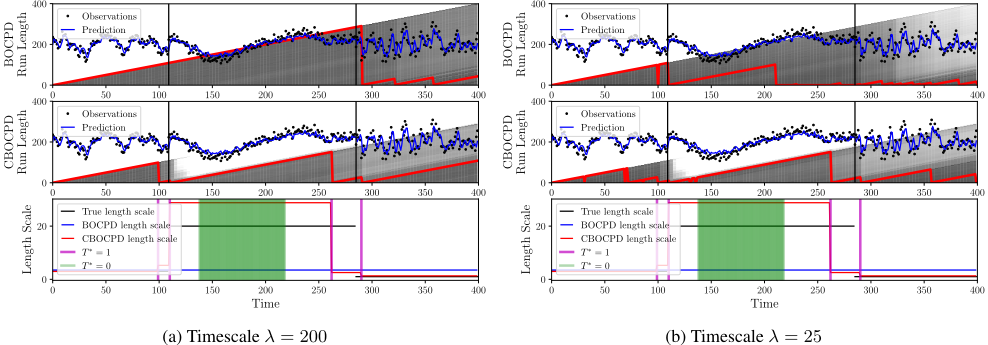
The BOCPD framework efficiently determines changes in GP modeling. The change is modeled by considering all the possible run lengths. One of the main assumptions of this framework is that parameters such as the kernel parameters or the hazard function do not change. However, this online CPD framework is vulnerable to the parameters, because inappropriate parameters degrade predictive performance on non-stationary data leading imprecise run length distribution as shown in Figure 2.
4.2 Confirmatory BOCPD
Algorithm 1 presents a theoretically justified online change detection algorithm, CBOCPD. The main idea of CBOCPD is to overcome the limitations of the assumption that the run length is independent of the data. However, we claim that the first term in Equation (6) can be directly calculated by the LRT in Section 3.3. The first two lines in Algorithm 1 initialize the parameters. In lines 3-13, Equation (7) is altered as
Here, we have two LRTs, T0 = I (2L ≥ Rδ,H0 ) and T1 = I (2L ≥Rδ,H1 ), with thresholds in line 4. Empirical thresholds are used since the theoretically calculated thresholds in Lemmas 3.3 and 3.4 are not tight enough to use in practice. We further define T∗ = 1 if T1 = 1, and T0 = 1 and T∗ = 0 if T1 = 0 and T0 = 0. The LRTs are applied to the window around t with W = xt-m:t+m. τ ∗ is the time point in the window that maximizes the LR, τ ∗ = argmaxτ∈CW 2Lτ . Here CW ⊆ {t - m, ..., t + m} is a set of change point candidates for the window. If both LRTs at time τ ∗ pass
Algorithm 1 Confirmatory BOCPD
1: m, δ ← half window size, error bound for the LRT 2: P(x0) ←N(µprior, σ2 prior ) 3: for t ∈ [1, T] do 4: Rδ,H0 ,Rδ,H1 ← thresholds for T0 , T1 5: H ←Hconst 6: if m < t < T -m then 7: set window W = xt-m:t+m 8: 2Lτ ← the LR between H0 and H1,τ with data W 9: τ ∗ , 2L = argmaxτ∈CW 2Lτ , maxτ∈CW 2Lτ 10: if T1 = 1 and T0 = 1 and τ ∗ = t then 11: H ← 1 - δ 12: else if T1 = 0 and T0 = 0 then 13: H ← δ 14: π(r) t ←P(xt|x(r) t-1 ) 15: P(rt = rt-1+1, x1:t) ←P(rt-1, x1:t-1)π(r) t (1-H) 16: P(rt = 0, x1:t-1) ← ∑rt-1 P(rt-1, x1:t-1)π(r) t H 17: P(x1:t) ← ∑rt P(rt, x1:t) 18: P(rt|x1:t) ←P(rt, x1:t)/P(x1:t) 19: P(xt+1|x1:t) ← ∑rt P(xt+1|x(r) t )P(rt|x1:t)and τ ∗ coincides with t, we decide that t is a CP and set P(rt = 0|rt-1, x(r) t-1 ) = 1 - δ, which enhances the probability of change in the BOCPD framework. In contrast, if neither test passes, we strongly believe there is no change and reduce the probability of change in the BOCPD framework. This is why we name this algorithm Confirmatory BOCPD. We add τ ∗ = t to avoid situations where the same time point maximizes the LR in several consecutive windows, resulting in duplicate CPs. Lines 14-19 follow the BOCPD framework [Adams and MacKay, 2007].
4.3 Theoretical Analysis of CBOCPD
We present sufficient conditions under which CBOCPD provides the lower prediction error compared to BOCPD. Here, the prediction error is defined as the expected absolute difference between the predictive mean given the true run length and the predictive mean under BOCPD and CBOCPD at a (detected) CP t, as a good prediction at a CP is a key factor in overall performance. For simplicity, we denote the expected value of xt under BOCPD and CBOCPD as EBO[xt|x1:t-1] and ECBO[xt|x1:t-1], respectively. Further we define αi = 1 - PBO(rt-1 = i|x1:t-1) under BOCPD and βi = 1 - PCBO(rt-1 = i|x1:t-1) under CBOCPD.
Non-stationary Case
We first investigate the case where a change exists.
Theorem 4.1. Consider BOCPD (Sec. 4.1) and CBOCPD (Sec. 4.2) algorithms where CBOCPD uses two statistical tests T0 and T1 with type II error of δII 0 and δII 1 respectively. When there exists a CP at t with mean value of µ1 which satisfies
where E[xt|∅] indicates the expected value of xt with prior distribution, if
with α0 indicating the probability of the run length not to be zero, then the absolute error of expected value of CBOCPD at t is less than or equal to the one of BOCPD as
Stationary Case
Next, we investigate the case where a change does not exist.
Theorem 4.2. Consider BOCPD (Sec. 4.1) and CBOCPD (Sec. 4.2) algorithms where CBOCPD uses two statistical tests T0 and T1 with type I error of δI0 and δI1 respectively. When there exists a confirmed non-CP at t with mean value of µ2 which satisfies
with αt-1 and βt-1 indicating the probability of the run length not to be t-1 under BOCPD and CBOCPD respectively, then the absolute error of the expected value of CBOCPD at t is less than or equal to the one of BOCPD as
5 Experimental Evaluations
5.1 Synthetic Data
In this experiment, we investigate two synthetic datasets generated by GPs with changes in the length scale and the variance of a Radial Basis Function kernel, respectively. Observations are obtained by adding the white Gaussian noise with the variance σ2no = 0.1. For both datasets, two CPs are drawn uniformly from time intervals (75, 125) and (275, 325) with end time T = 400.
For the first experiment, the length scale l switches from 3 to 20 and from 20 to 1 with the variance σ2 = 1. For the second experiment, the variance σ2 switches from 1 to 4 and from 4 to 0.3 with the length scale l = 3. We compare the proposed CBOCPD with BOCPD and CS (CUSUM)-BOCPD. For BOCPD, we use a modified version of the stationary GPBOCPD [Saatc¸i et al., 2010] by fixing the timescale λ. CSBOCPD uses CUSUM instead of the our proposed LRT in Algorithm 1. For all algorithms, the timescale of λ = 200 is used.
Figure 2a and Figure 2b show that CBOCPD identifies the length scale change in the data with the help of statistical tests, whereas BOCPD captures the change too less or too many times. The first two columns in Table 1 present the quantitative results from 100 runs of each algorithm after training on the first 100 points and testing on the remaining 300 points. CBOCPD outperforms BOCPD in terms of both negative log-likelihood (NLL) and mean squared error (MSE). The differences in performances become larger when there is a stronger correlation among the samples.
| LEN-CHANGE | VAR-CHANGE | Gazebo:Env1 | Gazebo:Env2 | Gazebo:Env3 | ||||||
|---|---|---|---|---|---|---|---|---|---|---|
| Method | NLL | MSE | NLL | MSE | NLL | MSE | NLL | MSE | NLL | MSE |
| BOCPD | 0.99±0.38 | 0.47±0.32 | 1.13±0.61 | 0.55±0.58 | 2.07±0.51 | 0.14±0.05 | 2.24±0.48 | 0.57±0.26 | 0.28±0.12 | 0.11±0.03 |
| CS-BOCPD | 0.95±0.32 | 0.43±0.30 | 1.05±0.42 | 0.48±0.40 | -0.11±0.33 | 0.12±0.04 | 1.82±1.51 | 0.55±0.27 | 0.25±0.16 | 0.10±0.02 |
| CBOCPD | 0.79±0.33 | 0.34±0.24 | 0.89±0.36 | 0.41±0.34 | -0.31±0.34 | 0.11±0.04 | 0.69±0.36 | 0.45±0.19 | -0.99±0.47 | 0.10±0.04 |
| Method | NLL | p-value | MSE | p-value |
|---|---|---|---|---|
| Nile Data (200 training points, 463 test points) | ||||
| ARGP ARGP-BOCPD GPTS BOCPD CBOCPD Well Log ARGP | 1.07±0.64 0.78±0.72 0.86±0.64 0.57±0.77 0.00±0.80 Data (500 7.20±0.60 0.00±0.30 | <0.0001 <0.0001 <0.0001 0.0014 N/A training <0.0001 N/A <0.0001 | 5.06±0.86 4.94±0.87 4.78±0.81 4.73±0.82 4.32±0.74 3050 test 17.3±2.6 4.68±0.46 8.27±0.61 | 0.0005 0.0017 0.0100 0.0115 N/A N/A |
| points, points) | ||||
| ARGP-BOCPD GPTS BOCPD CBOCPD Snow ARGP ARGP-BOCPD GPTS BOCPD CBOCPD | 3.73±0.42 4.35±0.31 0.30±0.27 | <0.0001 0.0010 | 19.2±1.3 4.92±0.44 test | <0.0001 <0.0001 <0.0001 0.2124 |
| (500 17.48±0.82 0.06±0.39 16.60±0.22 | points, | |||
| Data training 13380 points) | ||||
| 0.00±0.39 | <0.0001 <0.0001 <0.0001 N/A <0.0001 | 14.82±0.57 9.65±0.39 8.76±0.36 9.43±0.38 | <0.0001 <0.0001 <0.0001 N/A <0.0001 | |
CBOCPD 1.92±0.37 <0.0001 6.34±0.27 <0.0001
Table 2: Results of predictive performance on Nile data, Well Log Data and Snow Data. The results are provided with 95% of confidence interval and the p-value of the null hypothesis that a method is equivalent to the best performing method according to NLL, using a one sided t-test.
5.2 Gazebo Robot Simulation Data
We also conducted experiments on the Gazebo robot simulator to detect changes in the environment of a robot. We gathered data by moving the robot through a changing environment (i.e., varying ground properties). We used the Pioneer3AT robot with kinetic ROS. There are three environments. In the first environment (Env1), the ground changes at the midpoint from 'Plane ground' to 'Bumpy ground 1'. In the second environment (Env2), the robot moves from 'Bumpy ground 1' to 'Bumpy ground 2' where 'Bumpy ground 2' is more coarser than 'Bumpy ground 1'. Finally, in the third environment (Env3), the robot moves from 'Bumpy ground 2' back to the 'Plane ground'. For simplicity, we used only z-directional position data as the inputs. The last three columns in Table 1 show that CBOCPD outperforms other methods in all environments. Interestingly, the results show that CUSUM test does not help BOCPD much when the variance decreases as in Env3 but proposed LRT improves BOCPD in all the cases.
5.3 Real World Data
Further, we compare our proposed algorithm with autoregressive GP (ARGP), autoregressive GP with BOCPD (ARGPBOCPD), GP time series with BOCPD (BOCPD) and GP time series model (GPTS). For baseline methods we used the publicly available source codes 4 .
We first consider Nile data which records the lowest annual water levels on the Nile river during AD 622-1284 measured at the island of Roda. There is domain knowledge suggesting a CP in the year 715 due to the construction of a 'nilometer' [Popper, 1951; Balek, 1977]. Secondly, we used Well Log data which records 4050 nuclear magnetic resonance measurements while drilling a well. We also considered Snowfall data which records daily snowfall in Whistler, BC, Canada. In this dataset each method is evaluated by the ability to predict snowfall of next day using 35 years of test data.
Table 2 shows the predictive performance of our proposed algorithm compared to other GP based BOCPD methods. In Nile data, we see that combining BOCPD method with GP improves the performance. CBOCPD further improves the performance by leveraging the proposed statistical hypothesis tests and outperforms all other algorithms. In Well Log data, the nonlinear temporal correlations within each regime give a slight advantage to underlying predictive model of ARGP. However, CBOCPD still shows the competitive result. In Snowfall data, CBOCPD well detects the difference in noise levels and achieves the best performance in MSE.
6 Conclusion
This paper presents a novel framework for detecting changes in the covariance structure of the GP. We propose a online CPD algorithm, Confirmatory BOCPD, which is an improved version of BOCPD with statistical hypothesis tests. Experiments using synthetic and real-world datasets demonstrate that CBOCPD outperforms conventional BOCPDs.
Acknowledgments
This work was supported by the Industrial Convergence Core Technology Development Program funded by the Ministry of Trade, Industry & Energy (MOTIE), Korea (No. 10063172, Development of robot intelligence technology for mobility with learning capability toward robust and seamless indoor and outdoor autonomous navigation) and Institute for Information & communications Technology Planning & Evaluation (IITP) grant funded by the Ministry of Science and ICT (MSIT), Korea (No. 2017-0-01779, A machine learning and statistical inference framework for explainable artificial intelligence).
4 https://sites.google.com/site/wwwturnercomputingcom/ software/ThesisCodeAndData.zip
@inproceedings{ijcai2019p340,
  title     = {Confirmatory Bayesian Online Change Point Detection in the Covariance Structure of Gaussian Processes},
  author    = {Han, Jiyeon and Lee, Kyowoon and Tong, Anh and Choi, Jaesik},
  booktitle = {Proceedings of the Twenty-Eighth International Joint Conference on
               Artificial Intelligence, {IJCAI-19}},
  publisher = {International Joint Conferences on Artificial Intelligence Organization},
  editor    = {Sarit Kraus},
  pages     = {2449--2455},
  year      = {2019},
  month     = {8},
  note      = {Main track},
  doi       = {10.24963/ijcai.2019/340},
  url       = {https://doi.org/10.24963/ijcai.2019/340},
}
TY - CPAPER TI - Confirmatory Bayesian Online Change Point Detection in the Covariance Structure of Gaussian Processes AU - Han, Jiyeon AU - Lee, Kyowoon AU - Tong, Anh AU - Choi, Jaesik T2 - Proceedings of the Twenty-Eighth International Joint Conference on Artificial Intelligence, IJCAI-19 PB - International Joint Conferences on Artificial Intelligence Organization PY - 2019 SP - 2449 EP - 2455 DO - 10.24963/ijcai.2019/340 UR - https://doi.org/10.24963/ijcai.2019/340 ER -Copied
Machine-readable versions of this paper, for tools and AI agents:





