Conditions on Features for Temporal Difference-Like Methods to Converge

1 Introduction

A longstanding goal in reinforcement learning (RL) has been to find algorithms with linear function approximation that reliably converge to the fixed point of the Bellman equations. As such the convergence of different RL methods that display such characteristics have been researched extensively. The TD(λ) algorithm converges in an on-policy learning setting to the fixed point of a projected λ-weighted Bellman equation [Tsitsiklis and Van Roy, 1997]. The Residual Gradient algorithm is shown to minimise the Bellman error but suffers from double sampling [Baird, 1995]. More recently, some temporal difference-based methods have been shown to converge with off-policy learning. The GTD2 and TDC algorithms are shown to converge to the TD(0) solution under an off-policy learning setting [Sutton et al., 2009]. These algorithms have also been extended to their bootstrapped version GTD(λ) and shown to converge to the TD(λ) solution [Maei, 2011]. However, a core tenet in almost all of these convergence results is the assumption that these RL methods converge to a unique solution; for example in the proof of GTD2's convergence, the matrix quantities A and C are assumed to be non-singular, allowing for uniqueness of solution [Sutton et al., 2009, Theorem 1].

In addition to the convergence results, pertinent counterexamples have been documented in the literature that highlight how the choice of features is crucial to convergence of RL methods [Gordon, 1995; Tsitsiklis and Van Roy, 1996; Baird, 1995; Bertsekas, 1995; Boyan and Moore, 1995]. Bertsekas showed that TD(λ) with function approximation may converge to a parameter vector which generates a poor estimate of the value function (in terms of Euclidean distance) [Bertsekas, 1995]. Tsitsiklis and Van Roy provided a counter-example showing that RL methods may diverge even when the value function is representable by the chosen features [Tsitsiklis and Van Roy, 1996]. More recently, Sutton and Barto present a counter-example where methods that minimise the Bellman error may fail to learn the correct parameter value [Sutton and Barto, 2018, Example 11.4].

In this paper, we provide a complete characterization of non-uniqueness and the potential to converge to the wrong solution for a large class of RL algorithms we call natural algorithms. A natural algorithm is any method that can be characterized as solving for the unique fixed point (when it exists) of a projected Bellman equation. We consider all oblique projections and a Bellman equation based on the TD(λ) Bellman operator presented in [Tsitsiklis and Van Roy, 1997]. Under this definition, the natural algorithms include a large spectrum of algorithms: on one end of the spectrum, the natural algorithms include bootstrapped methods such as TD(λ) and GTD(λ) since they are characterized by an orthogonal projection, and on the other end the natural algorithms include Bellman-error based methods which are characterized by the identity projection. We consider an RL setting with a continuous state space S and finite action space A; note that a finite state space is a special case of our setup. Furthermore, we consider the infinite horizon problem for our results.

Our main contribution is to prove that natural algorithms, even under the setting where the value function can be represented exactly by the features, are inherently prone to nonuniqueness and will converge to the wrong solution for most feature choices. Our main result is as follows:

Theorem 5.1. Natural algorithms converge if and only if all non-zero linear combination of the features achieve their extreme values on a sub-region of the state space that has nonzero measure under the stationary distribution.

Importantly, given our characterisation, we provide some guidelines for choosing features and algorithms to avoid nonuniqueness. We show that state aggregation based features are a safe choice. We also provide a sufficient condition for algorithms to converge under other feature constructions.

This paper is organized as follows. In Section 2, we introduce some background and notation. In Section 3, we present the theory behind projected equation methods and the characteristic equation to projected Bellman equations. In Section 4, we present a detailed look at the counter-example presented by Sutton and Barto that demonstrates the non-uniqueness issues which plague Bellman-error methods [Sutton and Barto, 2018]. In Section 5, we present our main results and discuss their implications, including positive feature construction examples. In Section 6, we present our framework for analyzing convergence. Finally, in Section 7, we present the idea behind the proof of Theorem 5.1. For brevity, most proofs and supporting results have been omitted. However, the supporting results and omitted proofs can be found in the extended version of the paper [Hutter et al., 2019].

2 Background and Notation

We now reiterate some background RL concepts, mathematical concepts and notation used throughout this paper.

2.1 RL in Continuous State Space

We consider an agent-environment setup [Sutton and Barto, 2018] where an agent follows a stationary policy π and interacts with a Markov Decision Process (MDP). We assume a continuous state space S that is compact and measurable and a finite action space A. For simplicity, we will assume that S = R in all our examples. The expected reward function is a function R : S → R and represents the expected reward to be received for a given state following π. At a state s ∈ S, we assume that there is a transition density function T : S × S → [0, 1] whilst following π. Combined with an initial state s0, the state sequence can be viewed as a time-homogeneous Markov process with transition kernel defined by T(B|x) = ∫B T(y|x)dy , ∀B ∈ B(S) , x ∈ S where B(S) is the Borel sigma-algebra. We consider the infinite horizon problem and thus the value function at state s ∈ S is defined as the total discounted expected return: V (s) = E[∑∞t=0 γ tR(st)|s0 = s], where γ ∈ [0, 1) is the discount factor. By standard MDP theory, the value function satisfies the Bellman equation given by

for any state s ∈ S. The Bellman operator T : RS → RS is an affine linear operator on RS and is defined accordingly as

If we define PT to be an operator such that (PTf)(s) := ∫S T(s′ |s)f(s′ )ds′ , we can express the Bellman operator compactly as T V := R + γPTV for any V ∈ RS . The Bellman equation can then be expressed as the fixed point equation V = T V .

For an agent following a policy π and interacting with an MDP, the state sequence can be viewed as a Markov process with transition density function T. Throughout this paper we assume that the state Markov process admits a stationary measure µ. Under these assumptions, the value function space inherits extra geometric structure via an inner product defined with respect to µ. For any f, g ∈ RS ,

Showing that 〈·, ·〉µ is an inner product is routine. We define the norm on the associated inner product space by ‖·‖µ = √〈·, ·〉µ. The set of functions in the value function space with finite ‖·‖µ -norm is given by L2 (S, µ) := {V ∈ RS : ‖V ‖µ < ∞}. Under our assumptions, it can be shown that the value function associated with the Markov process lives in L2 (S, µ). Furthermore, our approximations ˆ V of V also evolve in this space. For any two functions V, ˜ V ∈ L2 (S, µ) we say that V is µ-orthogonal to ˜ V , denoted by V ⊥µ ˜ V , if and only if 〈V, ˜ V 〉µ = 0.

2.2 Linear Function Approximation

When using linear function approximation, the value function V is approximated by a linear combination of the features chosen from a finite-dimensional subspace of L2 (S, µ). Formally, the approximate value function ˆ V can be written as a linear combination ˆ V (s,w) = ∑ki=0 φi(s)wi, ∀s ∈ S where w = (w1,w2, . . . ,wk)⊤ ∈ Rk is a parameter vector and Φ = {φ1, . . . , φk} is the set of features from S to R such that span(Φ) is a finite-dimensional subspace of L2 (S, µ). To simplify notation, let us define φ(s) = (φ1(s), φ2(s), . . . , φk(s))⊤. The approximation ˆ V can then be represented compactly as an Euclidean inner product ˆ V (s,w) = 〈φ(s),w〉 = φ⊤(s)w. We now define a property of linear combination of features that will be crucial in characterizing non-uniqueness.

Definition 2.1 (Flat Extrema). Let ϕ be any linear combination of the features Φ, i.e. ϕ ∈ span(Φ), such that ϕ ̸≡ 0, ϕmax := maxs∈S ϕ(s) and ϕmin := mins∈S ϕ(s). Let Nα := {s : ϕ(s) ≥ αϕmax} for α ∈ [0, 1]. Then we say that ϕ has a flat maximum if µ[N1] := ∫N1 µ(s)ds > 0. Conversely, we say that ϕ has a non-flat maximum if µ[N1] = 0. Similarly, we define N - α := {s : ϕ(s) ≤ αϕmin} and say that ϕ has a flat minimum if µ[N - 1 ] > 0 and a non-flat minimum if µ[N - 1 ] = 0.

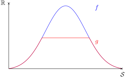
Any linear combination of features that have flat extrema achieve their maximum (and minimum) values in regions of the state space with non-zero measure under the stationary distribution µ. Conversely, linear combinations that have non-flat extrema achieve their maximum (and minimum) values in regions of the state space with measure zero. This corresponds to sub-regions of the state space that are never visited. Figure 1 gives an idea of what functions with a flat or non-flat maximum may look like.

2.3 The TD(λ) Operator

Tsitsiklis and Van Roy define the TD(λ) operator T (λ) in [Tsitsiklis and Van Roy, 1997] which we will adapt for our setting and derive a more compact form of the Bellman equation. For λ ∈ [0, 1), the TD(λ) operator T (λ) : L2 (S, µ) → L2 (S, µ) is given by

where V ∈ L2 (S, µ) and s ∈ S. As Tsitsiklis and Van Roy show, the TD(λ) operator can also be expressed as

[Tsitsiklis and Van Roy, 1997, Lemma 3]. We express this operator in a more compact form as

where

The P (λ) T operator can be seen as being a geometric average over the powers of PT . We define a λ-weighted discount factor G that corresponds to the discounting performed by the P (λ) T operator:

Clearly G is bounded in [0, 1). It is also important to note that for λ = 0 we recover the original discount factor of γ.

As we will see later, our class of natural algorithms consists of methods that look to converge to the fixed point of a projected Bellman equation

where Π is a projection operator.

3 Projected EquationMethods

We now introduce the theory of projected equation methods and present the characteristic equation of projected Bellman equations. We note that Bertsekas similarly covers projected Bellman equation methods [Bertsekas, 2011]. However, we find it useful to reiterate the concepts here as it pertains to a continuous state space and our setup.

3.1 Oblique Projection Operators

We consider the set of possible projection operators that can be applied to the Bellman equations to find an approximate solution. The projection operators that can project in any direction are collectively known as oblique projections. An oblique projection operator Π : L2 (S, µ) → L2 (S, µ) can be characterised as projecting onto im(Π), the image of Π, and orthogonally to im(Π∗ ) where Π∗ is the adjoint operator of Π. The purpose of looking at projection operators is to find learnable, finite-dimensional representations of the value function. Thus, we will focus on oblique projection operators with finite-dimensional image. For bounded projection operators with finite-dimensional image, the image of the adjoint has the same dimension.

Proposition 3.1 (Finite-Dimensional Projections). Let Π : L2 (S, µ) → L2 (S, µ) be a bounded linear operator with finite-dimensional image and let Π∗ be its adjoint. Then the image of Π∗ has the same dimension as the image of Π.

Proposition 3.1 allows us to characterise the oblique projection operators in terms of two finite-dimensional subspaces. We will generalise slightly beyond bounded projection operators by considering the case where the image of the adjoint is still finite-dimensional but may not be of the same dimension as the original projection operator. As we discuss in the next sub-section, this will allow us to express the solution to projected Bellman equations as a system of linear equations. We define the set of projection operators that we are interested in as follows.

Definition 3.2 (Finite Rank Projection Operators). Let Φ = {φ1, ..., φk} and Ψ = {ψ1, ..., ψn}. Let Π : L2 (S, µ) → L2 (S, µ) be an oblique projection operator such that im(Π) = span(Φ) and im(Π∗ ) = span(Ψ). Then Π can be characterised by the two sets (Φ, Ψ).

When conducting our analysis, we always assume the following.

Assumption 1. Let Ψ = {ψ1, . . . , ψn} be a basis for im(Π∗ ). Also, assume that ‖ψ‖1,µ := ∫S ψi(s)µ(s)ds = 1 for all i.

Note that Assumption 1 results in no loss of generality. Such a basis always exists for finite-dimensional spaces. Furthermore requiring ‖ψi‖1,µ = 1 is not restrictive. Since ψi ∈ im(Π∗ ) and im(Π∗ ) ⊂ L2 (S, µ), we must have that ‖ψi‖µ < ∞, implying that ‖ψi‖1,µ is also bounded and can be normalized. In the next sub-section we present the natural algorithms and how the solution to projected Bellman equations is characterised.

3.2 Natural Algorithms and the Solution to Projected Bellman Equations

We now look to determine the approximate value function ˆ V = φ⊤w ∈ span(Φ) found as the fixed point of a projected Bellman equation. For this task, it is natural to consider a finite rank projection operator Π characterised by (Φ,Ψ) to find ˆ V as the fixed point of ˆ V = ΠT (λ) ˆ V . Since the basis functions are known, the only task left is to find an expression for the parameter vector w. The following proposition states that w is the solution to a system of linear equations.

Proposition 3.3 (Characteristic Equation for Projected Bellman Equations). Let Π be a finite rank projection operator characterised by (Φ,Ψ). Suppose a unique solution exists and let ˆ V ∈ span(Φ), given by ˆ V = φ⊤w, be the unique fixed point of the projected Bellman equation

Let A ∈ Rn×k , B ∈ Rn×k , and b ∈ Rn be defined by

respectively for i = 1, 2, . . . , n and j = 1, 2, . . . , k. Then the parameter vector w = (w1, . . . , wk)⊤ is given as the solution to the system of linear equations

Proposition 3.3 suggests that any algorithm that converges to the fixed point of a projected Bellman equation in the limit has its solution characterised by the three matrix-vector quantities A,B, and b. We denote this class of algorithms as natural algorithms.

Definition 3.4 (Natural Algorithms). Let Π be a finite rank projection operator. If an algorithm converges to the fixed point ˆ V = φ⊤w of a projected Bellman equation

then the algorithm is a natural algorithm.

Some examples of natural algorithms are the TD(λ), GTD(λ) and Residual Gradient algorithms. This can be seen since both the TD(λ) and GTD(λ) algorithms converge to the TD(λ) solution and the Residual Gradient algorithm was shown explicitly to solve an obliquely projected Bellman equation [Tsitsiklis and Van Roy, 1997; Maei, 2011; Scherrer, 2010].

4 ACounter-Example to Uniqueness

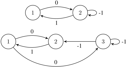
To motivate our results, we first present a counter-example highlighting some of the non-uniqueness issues that natural algorithms can face. Sutton and Barto provide a counterexample that highlights where Bellman-error based methods do not converge and experience non-uniqueness [Sutton and Barto, 2018, Example 11.4]. The counter-example considers the two Markov decision processes depicted in Figure 2. The edges indicate a state transition and the labels indicate the reward received. When two edges leave a single state, we assume the transition occur with equal probability. The transition matrices of MDP 1 and MDP 2 are then given by

The stationary distributions are given by µ1 = ( 13 , 2 3 )⊤ and µ2 = ( 13 , 1 3 , 13 )⊤ for MDP 1 and MDP 2 respectively. A simple linear function approximation mechanism is used with a two component parameter vector w = (w1,w2)⊤. In MDP 1, the value function can be represented exactly by ˆ V (1) = w1, ˆ V (2) = w2. In MDP 2, we assume that states 2 and 3 share a parameter value, giving ˆ V (1) = w1, ˆ V (2) = ˆ V (3) = w2. To any RL algorithm using this feature construction, the two MDPs appear indistinguishable as the feature-reward sequence generated under the stationary distribution occur with the same probabilities. Furthermore the Bellman error, given by EBE := ∥∥(I - γT )Φ ˆw - R∥∥2µ , is not a unique function of the data sample. For a parameter value ˆw = 0, the Bellman error is 0 inMDP 1 whilst it is 23 inMDP 2. This suggests that even though an algorithm minimizing the Bellman error may converge, it may converge to the wrong parameter vector.

In light of this example, we explicitly define a stronger notion of convergence to the correct solution. The next assumption asserts that there is a true environment and that the value function can be represented.

Assumption 2. Let R∗ , T ∗ be the true environment and assume that there exists a parameter vector w∗ such that the value function V ∗ can be represented as V ∗ (s) = φ⊤(s)w∗ .

We now define convergence as follows.

Definition 4.1. (Convergence) An algorithm is said to converge if it converges to w∗ or, equivalently, V ∗ .

5 Main Results

We now present our main results and discuss their implications. Our main theorem directly characterises convergence in terms of a property on the features.

Theorem 5.1 (Flatness Condition on Features). Natural algorithms converge if and only if all linear combinations of the features Φ have flat extrema.

It is important to note that Theorem 5.1 holds for all finite rank projections onto span(Φ). The factor determining convergence is the choice of features. Theorem 5.1 provides a restrictive condition on the possible feature choices available for natural algorithms with linear function approximation to converge. Not only are the usual assumptions of linear independence in the features necessary; it is required that all linear combinations of the features have flat extrema.

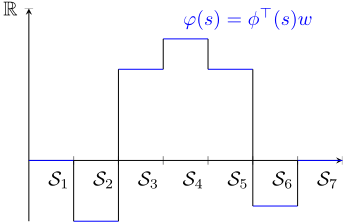
An immediate consequence of Theorem 5.1 is that state aggregation methods are always safe feature construction choices. If states are aggregated such that each subset has non-zero measure under the stationary measure, all value functions in the span of these features have flat extrema. An example of this is a partitioning-based state aggregation scheme, shown in Figure 3, that visibly has flat extrema. If there exist aggregated states with measure zero, these states would be unobserved under the stationary measure and would not impact the representation. This result is summarised in the following corollary.

Corollary 5.2 (State Aggregation). State aggregation is a safe feature construction choice for natural algorithms.

Though state aggregation is a sufficient choice for natural algorithms to avoid convergence issues, algorithms with other feature constructions have been shown to converge [Tsitsiklis and Van Roy, 1996]. We present a condition in the next subsection to help determine and construct convergent natural algorithms.

5.1 A Projection Perspective

Under Assumption 1, the inner product between ψi and any function ϕ ∈ span(Φ) can be seen as the projection of ϕ onto ψi. Our next result presents a condition on these projections which can aid in determining convergent algorithms with feature constructions other than state aggregation.

Theorem 5.3 (Convergent Natural Algorithms). All natural algorithms converge if and only if there exists an i such that for all ϕ ∈ span(Φ)

where G is defined in (2).

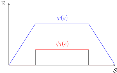
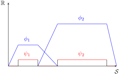
Theorem 5.3 guarantees a natural algorithm's convergence if it can project the extremal regions of any approximate value function. A simple case is when 〈ψi, ϕ〉µ = ϕmax or 〈ψi, ϕ〉µ = ϕmin. This occurs precisely when ϕ has flat extrema and ψi projects ϕ on the sub-regions of the state space where ϕ achieves its extremes. An example of this is shown in Figure 4.

Example 1. We now provide an explicit example of how Theorem 5.3 can help construct convergent natural algorithms. Consider the piece-wise linear features displayed in Figure 5. Any linear combination of these features also results in piece-wise linear functions that have flat maxima. Then any natural algorithm which has the functions ψi positive on the regions of the state space where the features achieve their flat maxima will satisfy Theorem 5.3. Effectively, such an algorithm disregards any information about the regions of the state space that are not in the flat maxima of the features. Such an algorithm can be determined without knowledge of the value function since it only depends on the features, which are chosen apriori.

Example 2. An example of a convergent natural algorithm that projects on the states that achieve the maximum value is the modified value iteration approach presented by Tsitsiklis and Van Roy [Tsitsiklis and Van Roy, 1996]. At the outset, K representative states s1, . . . , sK ∈ S are chosen and their feature vectors φ(s1), . . . , φ(sK) are constructed. The remaining states are then chosen from within the convex hull of the feature vectors of the representative states. In this manner, the feature construction ensures that the maximum value of all approximate value functions are centred on the representative states. The modified value iteration then solves for the fixed point of

where Φ† is the left inverse of Φ. In this construction, the projection operator is given by ΦΦ† . Since the nonrepresentative states are composed from the representative states, the algorithm proceeds by computing only on the representative states. Thus, this method effectively takes a projection on the points of the state space that achieve the maximum value.

6 Framework of Analysis

In this section we establish the framework we use for analysing convergence and non-uniqueness for natural algorithms. We call our framework the Bellman template. We specifically look to capture two phenomena of nonuniqueness that were displayed in Sutton and Barto's counterexample: how natural algorithms may converge to the wrong solution even when the value function is representable and how different MDP environments with different optimal parameter vectors appear indistinguishable under projection. We formally define the Bellman template as follows.

Definition 6.1 (Bellman Template). Let Π be a finite rank projection characterised by (Φ, Ψ). Let w ∈ Rk , R : S → R such that ‖R‖∞ < ∞, and T : S × S → [0, 1] such that ∫S T(s′ |s)ds′ = 1. The following constraints on (w,R, T) are collectively defined as the Bellman template:

• (w,R, T) satisfy the Bellman equation

where ˆ

· Let A ∈ Rn×k , B ∈ Rn×k and b ∈ Rn . R and T satisfy 〈ψi, φj〉µ = Aij , 〈ψi, P (λ) T φj〉µ = Bij , 〈ψi,R〉µ = bij for i = 1, . . . , n and j = 1, . . . , k respectively and w satisfies

We say that a triple (w,R, T) is a solution to the Bellman template if it satisfies these constraints.

A Bellman template solution represents an MDP environment (through the expected reward function R and the transition density function T) and its value function under the stationary policy (through the parameter vector w). The first constraint in the Bellman template restricts our attention to the case where the value function is exactly representable by the chosen features Φ. The second constraint provides a condition to capture when different solutions to the Bellman template appear indistinguishable under projection. In particular, we consider when different solutions (w,R, T) produce the same quantities A,B, and b that characterize solutions. It may seem strange that non-uniqueness could present an issue since a solution to a projected Bellman equation is uniquely determined by A, B and b. The crucial difference however is that we now let the environment variables, R and T , vary.

We define the condition of ambiguity, which represents non-uniqueness, as follows.

Definition 6.2 (Ambiguity). Ambiguity holds if the Bellman template has more than one (w, R, T) solution that have different parameters w.

Under ambiguity, different MDP environments with different optimal value functions appear the same to natural algorithms under projection. Therefore, natural algorithms fail to converge under ambiguity.

7 Theorem 5.1 Proof Idea

For brevity, we only present the key ideas behind the proof of Theorem 5.1 here. The full proof however can be found in the extended version of the paper [Hutter et al., 2019]. We first present a supporting result that characterises ambiguity.

Theorem 7.1. Let 0 ̸≡ ϕ ∈ span(Φ) and ϕmin := min s∈S ϕ(s) and ϕmax := max s∈S ϕ(s). Ambiguity holds if and only if there exists an f : S → [ϕmin, ϕmax] such that

for all i = 1, . . . , n, where χi(s) = ψi(s)µ(s) and G is defined in (2).

The idea behind the proof of Theorem 5.1 is to construct a function f that satisfies Theorem 7.1. We show that such a function f exists if and only if there exists a non-zero linear combination of the features that has non-flat extrema. Then by the equivalence given in Theorem 7.1, ambiguity holds meaning natural algorithms will fail to converge. Taking the contrapositive then gives Theorem 5.1.

To construct a suitable function, first consider the function ˜ f := 1G ϕ. Clearly ˜ f satisfies (5). For ϕmax < 0, ˜ f satisfies the upper bound on the range as ˜ f(s) ≤ ϕmax for all s ∈ S. Similarly, in the case where ϕmin > 0, ˜ f satisfies the lower bound on the range. However when ϕmax > 0, ˜ f exceeds the upper bound. Again in similar fashion, when ϕmin < 0, ˜ f exceeds the lower bound. We now look to construct a function from ˜ f that does not exceed the bounds in these cases whilst still satisfying (5). We will focus on the ϕmax > 0 case, noting that ϕmin < 0 is treated the same way. We consider capping ˜ f at Gϕmax and spreading the 'cut' pinnacle across the basis functions χi in a way that satisfies (5). Consider

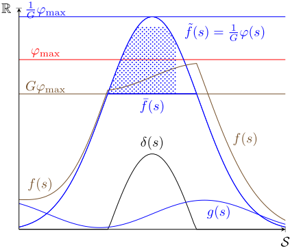
where δ(s) :=max{0, 1G ϕ(s)-Gϕmax} is the cut pinnacle. Now define f := ¯ f + g, where g is some function. We look to find g as the pinnacle δ projected onto the basis functions χi in such a way that (5) is satisfied. It can be shown that (5) is equivalent to

for all i = 1, . . . , n. Thus there are n constraints for g to satisfy. To get a gauge on whether spreading δ in this fashion may be possible, consider the following. The height of the portion of 1G ϕ that exceeds ϕmax is of order O(1 -G). Also, if ϕ has a non-flat maximum and G is sufficiently close to 1, this portion has 'mass' o(1 - G) since µ[NG] goes to 0 as G goes to 1. As g spreads the mass of δ over χi independently from G, it is of order o(1 - G). Thus for G sufficiently close to 1, g(s) < δ(s). Thus it seems plausible that f = ¯ f + g = 1G ϕ - δ + g would not surpass the upper bound of ϕmax. We employ an analogous construction to find a function f - that satisfies the lower bound for the case where ϕmin < 0. Finally, we are able to combine the different functions we construct to satisfy the range conditions for each case in Theorem 7.1 and ultimately show our result. Figure 6 provides a sketch of the construction we employ in this proof.

8 Conclusion

We have established that natural algorithms are inherently prone to fail without careful consideration of the choice of features. In particular, natural algorithms converge if and only if the features chosen only allow for linear combinations with flat extrema. We also presented a condition from a projection perspective that can help determine the convergence of natural algorithms as well. Given our results, we justify that state aggregation features are sufficient for all natural algorithms to converge. We also provide a condition under which natural algorithms with other feature constructions can converge if they project upon the extreme regions of the features. In doing so, we show how a convergent natural algorithm can be constructed from our result as well as arguing for the convergence of the modified value iteration approach presented in [Tsitsiklis and Van Roy, 1996].

It is important to note that our results begin where the assumptions in previous convergence proofs do not hold. As an example, TD(λ) is known to converge on-policy but counterexamples exist for the off-policy case [Tsitsiklis and Van Roy, 1997]. In our analysis, the off-policy case is subsumed by the projection operators we consider as we do not restrict them to be non-expansions with respect to the‖·‖µ -norm. Thus, our result also implies the divergence of Q-learning.

We note that the natural algorithm class, while extensive, does not cover all known RL algorithms with linear function approximation. In particular the ETD algorithm, introduced in [Sutton et al., 2016], does not fall within our natural algorithm class. The ETD algorithm includes an extra interest function i that alters the visiting probabilities of states, meaning we are no longer working with the stationary distribution µ.

An important factor in determining whether our results will hold in practice is the choice of discount factor. Throughout our analysis, the discount factor plays an important role in defining the extrema regions. As the discount factor moves away from one and towards zero, it becomes less likely that the non-flat extrema property will occur. Thus the discount factor determines the degree to which feature choices that deviate from flat extrema allow natural algorithms to converge. Also, our analysis centres on a strict notion of convergence to the true value function. Investigating whether our analysis can extend to characterise non-uniqueness when considering approximate value functions is an interesting open question.