
Hypergraph Induced Convolutional Manifold Networks
Proceedings of the Twenty-Eighth International Joint Conference on Artificial Intelligence. Main track. Pages 2670-2676.
https://doi.org/10.24963/ijcai.2019/371
Keywords
- Computer Vision: Computer Vision
- Machine Learning: Deep Learning
Abstract
Deep convolutional neural networks (DCNN) with manifold embedding have achieved considerable attention in computer vision. However, prior arts are usually based on the neighborhood-based graph modeling only the pairwise relationship between two samples, which fail to fully capture intra-class variations and thus suffer from severe performance loss for noisy data. While such intra-class variations can be well captured via sophisticated hypergraph structure, we are motivated and lead a hypergraph induced Convolutional Manifold Network (H-CMN) to significantly improve the representation capacity of DCNN for the complex data. Specifically, two innovative designs are provides: 1) our manifold preserving method is implemented based on a mini-batch, which can be efficiently plugged into the existing DCNN training pipelines and be scalable for large datasets; 2) a robust hypergraph is built for each mini-batch, which not only offers a strong robustness against typical noise, but also captures the variances from multiple features. Extensive experiments on the image classification task on large benchmarking datasets demonstrate that our model achieves much better performance than the state-of-the-art
- [Agarwal et al., 2005] Sameer Agarwal, Jongwoo Lim, Lihi Zelnik-Manor, Pietro Perona, David Kriegman, and Serge Belongie. Beyond pairwise clustering. In CVPR, vol- ume 2, pages 838-845, 2005.
- [Belkin et al., 2006] Mikhail Belkin, Partha Niyogi, and Vikas Sindhwani. Manifold regularization: A geometric framework for learning from labeled and unlabeled exam- ples. J. Mach. Learn. Res., 7:2399-2434, 2006.
- [Elhamifar and Vidal, 2013] Ehsan Elhamifar and Rene Vi- dal. Sparse subspace clustering: Algorithm, theory, and applications. IEEE Trans. Pattern Anal. Mach. Intell., 35(11):2765-2781, 2013.
- [Gao et al., 2013] Shenghua Gao, Ivor Wai-Hung Tsang, and Liang-Tien Chia. Laplacian sparse coding, hypergraph laplacian sparse coding, and applications. IEEE Trans. Pattern Anal. Mach. Intell., 35(1):92-104, 2013.
- [Gao et al., 2014] Yue Gao, Rongrong Ji, Peng Cui, Qiong- hai Dai, and Gang Hua. Hyperspectral image classification through bilayer graph-based learning. IEEE Trans. Image Process., 23(7):2769-2778, 2014.
- [Han et al., 2017] Bohyung Han, Jack Sim, and Hartwig Adam. Branchout: Regularization for online ensemble tracking with convolutional neural networks. In CVPR, pages 521-530, 2017.
- [He and Niyogi, 2003] Xiaofei He and Partha Niyogi. Local- ity preserving projections. In NIPS, pages 153-160, 2003.
- [He et al., 2016] Kaiming He, Xiangyu Zhang, Shaoqing Ren, and Jian Sun. Deep residual learning for image recog- nition. In CVPR, pages 770-778, 2016.
- [Howard et al., 2017] Andrew G. Howard, Menglong Zhu, Bo Chen, Dmitry Kalenichenko, Weijun Wang, Tobias Weyand, Marco Andreetto, and Hartwig Adam. Mo- bilenets: efficient convolutional neural networks for mo- bile vision applications. CoRR, abs/1704.04861, 2017.
- [Huang et al., 2010] Yuchi Huang, Qingshan Liu, Shaoting Zhang, and Dimitris N Metaxas. Image retrieval via prob- abilistic hypergraph ranking. In CVPR, pages 3376-3383, 2010.
- [Huang et al., 2015] Sheng Huang, Mohamed Elhoseiny, Ahmed Elgammal, and Dan Yang. Learning hypergraph- regularized attribute predictors. In CVPR, pages 409-417, 2015.
- [Krizhevsky, 2009] Alex Krizhevsky. Learning multiple lay- ers of features from tiny images. 2009.
- [Liu et al., 2013] Guangcan Liu, Zhouchen Lin, Shuicheng Yan, Ju Sun, Yong Yu, and Yi Ma. Robust recovery of sub- space structures by low-rank representation. IEEE Trans. Pattern Anal. Mach. Intell., 35(1):171-184, 2013.
- [Liu et al., 2017] Qingshan Liu, Yubao Sun, Cantian Wang, Tongliang Liu, and Dacheng Tao. Elastic net hypergraph learning for image clustering and semi-supervised classifi- cation. IEEE Trans. Image Process., 26(1):452-463, 2017.
- [Lu et al., 2015] Jiwen Lu, Gang Wang, Weihong Deng, Pierre Moulin, and Jie Zhou. Multi-manifold deep met- ric learning for image set classification. In CVPR, pages 1137-1145, 2015.
- [Netzer et al., 2012] Yuval Netzer, Tao Wang, Adam Coates, Alessandro Bissacco, Bo Wu, and Andrew Y Ng. Reading digits in natural images with unsupervised feature learn- ing. 2012.
- [Rifai et al., 2011] Salah Rifai, Yann N Dauphin, Pascal Vin- cent, Yoshua Bengio, and Xavier Muller. The manifold tangent classifier. In NIPS, pages 2294-2302, 2011.
- [Simonyan and Zisserman, 2014] Karen Simonyan and An- drew Zisserman. Two-stream convolutional networks for action recognition in videos. NIPS, 1(4):568-576, 2014.
- [Simonyan and Zisserman, 2015] Karen Simonyan and An- drew Zisserman. Very deep convolutional networks for large-scale image recognition. In ICLR, 2015.
- [Szegedy et al., 2016] Christian Szegedy, Sergey Ioffe, Vin- cent Vanhoucke, and Alexander A Alemi. Inception-v4, inception-resnet and the impact of residual connections on learning. pages 4278-4284, 2016.
- [Tomar and Rose, 2014] Vikrant Singh Tomar and Richard C Rose. Manifold regularized deep neural networks. In In- terspeech, 2014.
- [Wang et al., 2015a] Limin Wang, Yu Qiao, and Xiaoou Tang. Action recognition with trajectory-pooled deep- convolutional descriptors. In CVPR, pages 4305-4314, 2015.
- [Wang et al., 2015b] Meng Wang, Xueliang Liu, and Xin- dong Wu. Visual classification by ℓ 1 -hypergraph model- ing. IEEE Trans. Knowl. Data Eng., 27(9):2564-2574, 2015.
- [Wen et al., 2016a] Yandong Wen, Zhifeng Li, and Yu Qiao. Latent factor guided convolutional neural networks for age-invariant face recognition. In CVPR, pages 4893- 4901, 2016.
- [Wen et al., 2016b] Yandong Wen, Kaipeng Zhang, Zhifeng Li, and Yu Qiao. A discriminative feature learning ap- proach for deep face recognition. In ECCV, pages 499- 515, 2016.
- [Yang et al., 2017] Shijie Yang, Liang Li, Shuhui Wang, Weigang Zhang, and Qingming Huang. A graph regular- ized deep neural network for unsupervised image repre- sentation learning. In CVPR, pages 7053-7061, 2017.
- [Yuan et al., 2015] Yuan Yuan, Lichao Mou, and Xiaoqiang Lu. Scene recognition by manifold regularized deep learn- ing architecture. IEEE Trans. Neural Netw., 26(10):2222- 2233, 2015.
- [Zagoruyko and Komodakis, 2016] Sergey Zagoruyko and Nikos Komodakis. Wide residual networks. In BMVC, 2016.
- [Zhang et al., 2017] Zhihong Zhang, Lu Bai, Yuanheng Liang, and Edwin Hancock. Joint hypergraph learning and sparse regression for feature selection. Pattern Recognit., 63:291-309, 2017.
References were extracted automatically from the PDF and may contain errors.
Full text extracted automatically from the PDF; figures, tables and equations may differ. The PDF is the version of record.
1 Introduction
Deep learning models with convolutional neural networks have been widely applied to various classification problems such as image classification [He et al., 2016], action recognition [Simonyan and Zisserman, 2014; Wang et al., 2015a] and object tracking [Han et al., 2017]. A typical CNN adopts the softmax loss to train a classification model, which can well discriminate the inter-class samples. However, when facing the data with large intra-class variations, the performance of the traditional CNN models degenerates dramatically. The center loss [Wen et al., 2016a] made an attempt to leverage the prior of data distribution to enforce the deep features from the same class to have small intra-class variance, which assumes that the data follows Gaussian distributions.
∗Corresponding Author
However, for many real-world problems, the Gaussian assumption usually does not hold. Amore natural thought is to adopt manifold data preserving techniques [Gao et al., 2013; Rifai et al., 2011] to address the robustness issue for the noisy data in real applications.
Despite the exciting progress, incorporating manifold preserving method into deep models still remains as an open problem. In [Yuan et al., 2015], researchers [Yuan et al., 2015] adopt manifold learning as a base unit plugged into a deep architecture, which indeed works but suffers from a huge computational burden. While Graph Regularized Deep Neural Network (GR-DNN) [Yang et al., 2017] endues the traditional Deep Auto-Encoder with the ability to preserve the local geometric structure of the data. Multi-Manifold Deep Metric Learning (MMDML) [Lu et al., 2015] transforms multiple sets of nonlinear transformations to a shared feature subspace to maximize the manifold margin of different classes. Manifold Regularized Deep Neural Networks (MRDNN) [Tomar and Rose, 2014] attempts to make the associated techniques preserve the underlying manifold based relationships amongst speech feature vectors.
The previous methods are usually applied to image /speech datasets of the small or middle sizes, since the graph construction is intractable for the large-scale data. Thus, how to embed the data correlations into the training pipeline of deep learning is still an open problem. Specifically, the existing methods usually adopt the neighborhood-based graph to preserve the structure of the data, which is sensitive to noise and performs worse when facing the badly corrupted noisy data. That may be the reason that previous method can not well explore the real-world data, and only limited improvements are achieved in practical applications. We note that compared with the neighborhood-based graph, the robust graph construction methods such as low-rank graph [Liu et al., 2013] or ℓ1-graph [Elhamifar and Vidal, 2013] needs more computational resources. Therefore, these robust graphs cannot be applied to deep learning models. The manifold-based robust deep learning can be further boosted by exploring more about the local structure of data.
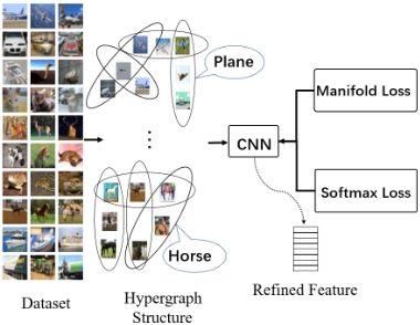
In this paper, we propose a hypergraph induced Convolutional Manifold Networks (H-CMN). The main difference between our model and the previous methods lies in that ours can scale to the large-scale datasets such as ImageNet and at the same time gain more robustness on the noisy data by introducing the hypergraph learning into deep learning training pipeline. Besides, our model simultaneously captures the variations of multiple deep features by constructing a hypergraph on each mini-batch iteration of the training pipeline. Figure 1 shows the motivation of our model.
The highlights of our proposed H-CMN model are summarized as follows:
- Our model is flexible and efficient for the large-scale dataset such as ImageNet by constructing a hypergraph in each mini-batch.
- The constructed hypergraph is not only robust to the noise, but also able to simultaneously capture the variations of multiple deep features.
- The extensive experiments on large-scale datasets validate the superior performance of the proposed model over the state-of-the-arts. In particular, the performance is significantly improved for noisy data.
2 Hypergraph InducedManifold Networks
We assume a training dataset of N samples, X = {x1 , x2 , · · · , xi , · · · , xN }, where xi is the i-th sample with the class label, Ri, and N is the number of samples.
2.1 Manifold Loss Based on Hypergraph
We propose to adopt a hypergraph to represent the local neighborhood structure for the samples in each mini-batch, where each hyperedge in the hypergraph can link more than two vertices [Agarwal et al., 2005]. Thus, the high-order relationships of the data are effectively modeled by a hypergraph. Hypergraph has been applied to various tasks such as image retrieval [Huang et al., 2010] and attribute predicting [Huang et al., 2015] and hyperspectral image classification [Gao et al., 2014].
Suppose a hypergraph G = (V,E,W) is composed of a vertex set V , a hyperedge set E, and a weights matrix of hyperedges W, where the weight of a hyperedge e is represented as w(e). A hypergraph can be represented by an incidence matrix H indicating whether a vertex is connected by a corresponding hyperedge, or not. The widely used binary incidence matrix is defined as: H(v, e) = 1 if v ∈ e; otherwise H(v, e) = 0. Based on the incidence matrix H and hyperedge weights W, the edge degree of each hyperedge e is defined as δ(e) = ∑e∈E H(v, e).
By incorporating a hypergraph, the proposed manifold loss is defined as
where fQ(xi) is the CNN deep feature of the i-th sample, which is directly related to the learned filters (Q) and Aij is the similarity between two samples xi and xj, which is defined as
where w(e) is the hyperedge weight and δ(e) is the edge degree of the hyperedge e.
By minimizing the manifold loss, the deep features can reflect the local neighborhood structure of the data samples within each hyperedge.
2.2 Manifold-aware Training Loss
Our proposed model combines the manifold loss and the softmax loss, resulting in the following training loss:
where the first component is the softmax loss, designed to enlarge the inter-class differences. θ denotes the weight matrix in the last fully connected (FC) layer. γ is the weight decay coefficient. The second component is the manifold loss, which is particularly designed for large intra-class variations. ρ is the regularization parameter to trade-off two training losses.
For the DCNN-based deep learning models 1 , the deep features are passed to the last Fully Connected (FC)-layer for the label prediction. For simplicity, we assume the CNN model has one FC-layer. fQ(xi) is the deep features of xi, belonging to the Ri-th class and Q is the filter weights, and θ is the weights matrix in the last FC layer. The softmax metric for the predicted probability of the Ri-th class is defined as
1 In this paper, the typical DCNN-based deep learning models include VGG [Simonyan and Zisserman, 2015], GoogLeNet [Szegedy et al., 2016] , WideResNet [Zagoruyko and Komodakis, 2016] and a light weight CNN-MobilNet [Howard et al., 2017].
where P is the number of data classes and θj is the j-th column of the weights matrix.
By minimizing the manifold aware training loss, our proposed H-CMN model learns the deep features, which not only reflect the simultaneous variances of multiple deep features on the manifold, but also enlarges the inter-class separability using the label supervisory information.
3 Fast Hypergraph Construction
3.1 The Main Idea
The manifold loss is identical to the manifold regularization [Belkin et al., 2006; He and Niyogi, 2003], which has been widely used in semi-supervised learning. However, how to embed manifold into a deep learning model is still an open problem that remains unsolved before our work. For deep learning model usually involves the large-scale dataset, it is intractable to directly adopt the existing hypergraph construction methods for hyperedge generation. To this end, both the neighborhood-based approach and the recent proposed representation-based approach [Liu et al., 2017; Wang et al., 2015b; Zhang et al., 2017] usually generate a set of hyperedges using the entire training set, which doesn't easily scale up for the large-scale data.
The training procedure of the deep learning model usually depends on the mini-batch Stochastic Gradient Descent (SGD) approach. For computational efficiency, it is crucial to embed a hypergraph into the SGD iterations. Therefore, we construct multiple class-specific feature buffers to store a small number of samples for each iteration, and then generate the hypergraph of the data using the samples in the feature buffers for reflecting the local neighborhood structure.
3.2 Mini-Batch Based Data Reconstruction
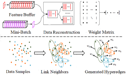
In the following, we give the details of how to construct a hypergraph for deep learning. Figure 2 gives a simple illustration of our proposed hypergraph construction procedure. For designing an efficient hypregraph construction to make the traditional SGD work, we construct multiple class-specific feature buffers for only storing the previous samples from the mini-batches of the last iterations. These chosen samples share the same class label. We assuming that the training set contains P classes of the samples, we construct P feature buffers with k0 size for storing a small number of samples in the training set.
Since the SGD training strategy optimizes the training loss in each mini-batch, we take one sample xi from the current mini-batch, and combine it into the corresponding classspecific feature buffer. Then, xi is taken as the center vertex and its k-nearest-neighbors from the corresponding classspecific feature buffer are chosen for further processing to generate one hyperedge of a hypergraph.
Note that xi may also be involved in the other hyperedges, whose center vertex is the k-nearest-neighbor of xi. Furthermore, for the k-nearest-neighbor xj of xi is taken as the center vertex to generate the correlated hyperedges by reconstructing xj by its the k-nearest-neighbors chosen from the corresponding class-specific feature buffer and xi. As a result, k+1 hyperedges are generated to capture the local neighborhood structures between xi and its k-nearest-neighbors from the corresponding class-specific feature buffer.
To generate a noise-resistant hyperedge set, we take center vertex and reconstruct it by its k-nearest-neighbors as
where xp is the center vertex. X∗p is the data matrix of the k-nearest-neighbors of xp. cp is the coefficients vector of the centroid vertex. λ is the regularization parameter to tradeoff between the data reconstruction term and the regularization.
The first term is the data reconstruction term, which represents center vertex as the linear combination of its k-nearestneighbors. The second term is the ℓ2-norm regularization, which has the following two advantages: (1) It makes the linear regression problem non-singular even if (X∗p )T (X∗p ) is not invertible for the case when the number of the nearest neighbors is much less than the number of the data samples. (2) It is suitable to choose the correlated samples as the vertices of each hyperedge, which has a group selection effect for the highly-correlated data.
Eq. (5) has the closed-form solution, which is derived as
Each entry in the coefficient matrix is obtained for modulating the data affinity. Here, each column of the coefficient matrix naturally characterizes how other samples contribute to the reconstruction of a given sample. Note that the noise component is separated from the original data and the clean data is represented as the linear combination of its k-nearest neighbors. The derived coefficients are robust to noise, while reflecting the local manifold structures of the data.
3.3 Fast Hyperedge Generation
To effectively capture the grouping and discriminative structures of the data, we only preserve those coefficients over a given threshold and make the coefficients under this threshold be zeros. Furthermore, the incidence relation between a hyperedge and its vertices, is defined as [Liu et al., 2017]:
where ep is the hyperedge associated with the center vertex xp, and cpj is the j-th coefficient of associated with xp and τ is the given threshold.
Hyperedge weighting is crucial for the learning task. We sum all the coefficients of vertices within a hyperedge as the hyperedge weight, which is defined as
For each sample in the current mini-batch, we repeat the aforementioned procedure to generate a set of hyperedges for the current mini-batch iteration. After finishing a mini-batch iteration, the samples in the current mini-batch is added to the corresponding queue of the class-specific feature buffer. Thus, the hypergraph construction is effectively embedded into each mini-batch-based SGD iteration.
The computational complexity of hypergraph construction is O(dk2N), where d is the data dimensionality, k is the neighborhood size parameter, and N is the number of samples. Since the neighborhood size is usually very small, the computation of the hypergraph construction is tractable for the SGD iterations.
4 Model Training
To embed the manifold loss into the CNN training, it is crucial to compute the manifold loss using the mini-batch for each iteration. In this article, we suppose the mini-batch size is M.
4.1 Computation of Manifold Loss
As shown in Eq. 3, the key step of computing the manifold loss is to measure the similarity Aij between two vertices vi(xi) and vi(xj), decided by the averaged neighboring affinities close to them, which is further affected by the hyperedges sharing two common vertices (vi and vi).
After a set of the hyperedges are generated for each minibatch, the number of the hyperedges is k + 1 for each sample in the current mini-batch. Thus, it is computationally tractable to visit each hyperedge to find whether the corresponding hyperedge contains two common samples. The aforementioned procedure is repeated to compute the manifold loss of mini-batch.
4.2 Update Rules
The update of the filter weights and the weights of the last FC-layer are iteratively processed. In each iteration, the filter weights and the weights of the last FC-layer are updated using mini-batch. Let the size of a mini-batch be M, Equre 3 is reformulated as
For the FC-layer, the weights matrix is updated by
Algorithm 1 Training of convolutional manifold networks
Input: The training set of the samples X Parameter: Initialized filter weights Q in the convolution layers, the weights matrix θ in the last FC-layer and the itera-
tion number t = 0
Output: The optimized parameters Q and θ
- 1: while not converged do
- 2: Step 1: t=t+1.
- 3: Step 2: Compute the joint loss, Jγ,ρ(θ,Q).
- 4: Step 3: Update θ(t+1) according to Eq. 10.
- 5: Step 4: Update Q(t+1) according to Eq. 11.
- 6: end while
where µ is the learning rate and t is the iteration number.
The filter weights for the convolutional layers, Q, is updated by
where Aij can be efficiently computed by the hypergraph construction for the current mini-batch iteration.
Algorithm 1 lists the main procedure of our proposed HCMNmodel. For the convergence of this iterative algorithm, because the computation of the manifold loss does not hurt the convergence of the training pipeline of the typical CNN, our model can be effectively trained using the SGD approach.
5 Experiments and Discussions
We used the typical DCNN as the backbone to train our model by SGD with only a small amount of parameter increase compared to the base model. In our experiments, VGG [Simonyan and Zisserman, 2015], WideResNet [Zagoruyko and Komodakis, 2016], GoogLeNet [Szegedy et al., 2016] and MobilNet [Howard et al., 2017] are chosen. For clarification, we refer to our method by adopting the VGG, GoogleNet and WideResNet and MobilNet as backbone as H-CMNV, HCMNG, H-CMNW and H-CMNM, respectively, where the feature buffer size is set to 100 and the neighborhood size parameter is set to 10. The compared deep learning models were trained on the 4 GPUs (Titan XP), which have 3.20G HZ and 12G memory. The mini-batch size is set to 150.
Furthermore, we compared our model to the state-ofthe-art methods: Center loss [Wen et al., 2016b] and the typical CNN model: VGG [Simonyan and Zisserman, 2015], GoogleNet [Szegedy et al., 2016] and WideResNet [Zagoruyko and Komodakis, 2016]. For fair comparisons, we use the default parameter settings such as the learning rate in their base model from all the compared methods. In our experiments, the number of the epochs for our model is set to be 180. Then, we run 5 times and report the Mean values and standard deviations (Std)
To understand how robust hypergraph affects the performance of deep learning model, we also used the neighborhood-based graph instead of a hypergraph to preserve the pairwise relationship between two deep features, where each sample is directly linked to its k-nearestneighbors. For clarity, we refer to the deep learning model using neighborhood-based graph as Gr-CNN.
For other deep manifold methods without open source code, they are not tested in following experiments. Note that Gr-CNN have a similar concept as other deep manifold methods, which thus can be used to validate our superior performance over conventional ones in the field.
5.1 Parameter Setting
Our model has four essential parameters: (1) the ℓ2-norm regularization parameter λ of ridge regression, (2) the trade-off parameter ρ between the softmax loss and the manifold loss, (3) the weight decay coefficient γ, and (4) the threshold parameter τ of the hyperedge generation. For the threshold parameter τ, we set the threshold parameter as the function of the largest coefficient of centroid sample, i.e., τ = τ s (cmax ), where cmax is the largest coefficient of the centroid sample. In addition, (1) the size of feature buffer k0 and (2) the neighborhood size k are also two issues that affect the performance.
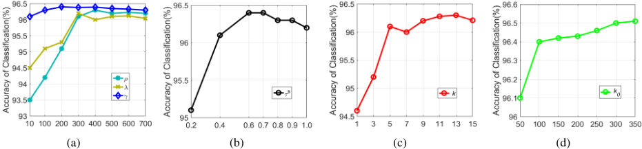
We conducted the classification experiments on the CIFAR-10 natural image dataset [Krizhevsky, 2009] to analyze how these parameters affect the classification performance. Figure 3 shows the results under different parameter values.
From Figure 3, we have the following observations:
As the trade-off parameter ρ increases, the performance increases accordingly. When ρ is larger than 300, the performance becomes stable.
The performance increases as the ℓ2-norm regularization parameter λ increases. The performance becomes stable when λ is larger than 500.
When the weight decay coefficient γ is ranged from 200 to 600, the performance becomes stable. For a small or a large parameter value, the performance degenerate slightly.
As the threshold parameter τ of hyperedge generation increases, the performance increases accordingly. When τ s is larger than 70% of the largest coefficient, the performance degenerates with a small gradient.
When the neighborhood size k is larger than 5, the performance is fairly stable. The experimental results shows that our model is insensitive to the large neighborhood sizes.
| Noise ratio | 0 | 10% | 30% | 50% |
|---|---|---|---|---|
| VGG | 96.6 (0.1) | 94.7 (0.1) | 89.7 (0.2) | 87.6 (0.3) |
| H-CMNV | 97.1 (0.2) | 95.3 (0.1) | 93.6 (0.1) | 90.4 (0.3) |
| GoogLeNet | 96.5 (0.2) | 94.8 (0.2) | 90.1 (0.3) | 87.9 (0.1) |
| H-CMNG | 97.2 (0.3) | 95.7 (0.1) | 93.3 (0.2) | 91.2 (0.3) |
| WideResNet | 97.2 (0.1) | 94.1 (0.2) | 90.7 (0.3) | 88.3 (0.3) |
| H-CMNW | 98.2 (0.0) | 97.3 (0.1) | 94.2 (0.1) | 93.8 (0.2) |
| Center Loss | 97.3 (0.3) | 95.3 (0.2) | 91.3 (0.1) | 89.5 (0.3) |
| Gr-CNN | 97.6 (0.0) | 95.1 (0.1) | 92.3 (0.2) | 90.6 (0.3) |
| Noise ratio | 0 | 10% | 30% | 50% |
|---|---|---|---|---|
| VGG | 93.6 (0.0) | 90.3 (0.2) | 87.8 (0.1) | 84.2 (0.1) |
| H-CMNV | 94.5 (0.2) | 93.1 (0.1) | 90.9 (0.0) | 88.8 (0.3) |
| GoogLeNet | 94.1 (0.2) | 91.2 (0.3) | 88.4 (0.1) | 85.3 (0.4) |
| H-CMNG | 95.1 (0.3) | 93.8 (0.2) | 92.0 (0.2) | 90.5 (0.1) |
| WideResNet | 94.5 (0.3) | 90.3 (0.4) | 88.6 (0.2) | 85.2 (0.3) |
| H-CMNW | 96.8 (0.2) | 94.8 (0.1) | 93.2 (0.3) | 91.9 (0.2) |
| Center Loss | 94.9 (0.3) | 91.6 (0.2) | 89.4 (0.2) | 86.7 (0.3) |
| Gr-CNN | 95.6 (0.2) | 92.8 (0.1) | 90.1 (0.3) | 87.6 (0.2) |
| Noise ratio | 0 | 10% | 30% | 50% |
|---|---|---|---|---|
| VGG | 73.5 (0.2) | 70.4 (0.3) | 67.1 (0.1) | 64.5 (0.3) |
| H-CMNV | 75.2 (0.2) | 73.4 (0.1) | 70.5 (0.0) | 68.9 (0.2) |
| GoogLeNet | 77.6 (0.4) | 74.2 (0.2) | 71.3 (0.0) | 69.8 (0.3) |
| H-CMNG | 80.5 (0.1) | 78.9 (0.1) | 76.8 (0.0) | 74.5 (0.2) |
| WideResNet | 77.3 (0.2) | 75.3 (0.3) | 73.1 (0.2) | 70.4 (0.2) |
| H-CMNW | 81.3 (0.2) | 80.4 (0.2) | 78.3 (0.0) | 76.9 (0.1) |
| Center Loss | 78.5 (0.3) | 77.4 (0.3) | 75.9 (0.2) | 71.7 (0.4) |
| Gr-CNN | 79.6 (0.3) | 78.9 (0.2) | 76.1 (0.3) | 73.2 (0.2) |
As the size of feature buffer k0 increases, performance increases slightly. However, the difference of the performance is small for different buffer sizes, since k0 is larger than 100.
| Noise ratio | 0 | 10% | 30% | 50% |
|---|---|---|---|---|
| MobileNet | 70.8 (0.4) | 68.1 (0.3) | 64.1 (0.3) | 58.3 (0.4) |
| H-CMNM | 72.9 (0.2) | 71.9 (0.3) | 70.8 (0.1) | 68.8 (0.4) |
| Center Loss | 69.5 (0.5) | 66.8 (0.4) | 64.3 (0.5) | 60.2 (0.4) |
| Gr-MNet | 72.0 (0.3) | 70.2 (0.4) | 66.4 (0.2) | 62.1 (0.5) |
| Dataset | SVHN | CIFAR10 | CIFAR100 | ImageNet |
|---|---|---|---|---|
| VGG | 0.0323 | 0.0285 | 0.0366 | N/A |
| H-CMNV | 0.1126 | 0.0749 | 0.1254 | N/A |
| GoogLeNet | 0.2857 | 0.2413 | 0.2352 | N/A |
| H-CMNG | 0.6028 | 0.6213 | 0.6128 | N/A |
| WideResNet | 0.3877 | 0.3998 | 0.2363 | N/A |
| H-CMNW | 1.1174 | 1.1164 | 1.0357 | N/A |
| Center Loss | 0.3934 | 0.3808 | 0.2385 | 0.8956 |
| Gr-CNN | 0.3364 | 0.4130 | 0.3490 | N/A |
| MobilNet | N/A | N/A | N/A | 0.9010 |
| H-CMNM | N/A | N/A | N/A | 2.3012 |
| Gr-MNet | N/A | N/A | N/A | 1.0164 |
| Dataset | SVHN | CIFAR10 | CIFAR100 | ImageNet |
|---|---|---|---|---|
| VGG | 0.006 | 0.012 | 0.012 | N/A |
| H-CMNV | 0.007 | 0.016 | 0.015 | N/A |
| GoogLeNet | 0.025 | 0.067 | 0.065 | N/A |
| H-CMNG | 0.032 | 0.074 | 0.073 | N/A |
| WideResNet | 0.61 | 0.53 | 0.59 | N/A |
| H-CMNW | 0.63 | 0.73 | 0.63 | N/A |
| Center Loss | 0.66 | 0.62 | 0.61 | 0.003 |
| Gr-CNN | 0.73 | 0.71 | 0.77 | N/A |
| MobilNet | N/A | N/A | N/A | 0.004 |
| H-CMNM | N/A | N/A | N/A | 0.005 |
| Gr-MNet | N/A | N/A | N/A | 0.004 |
5.2 Image Classification on Corrupted Data
The robustness to noise is crucial for deep features. To know how noise affects the performance, we conducted the classification experiments on the corrupted datasets, where the Gaussian noise is added to each image, x; that is, ˜x = x+αn, where α is the noise ratio ranging from 10% to 50% with an interval of 20%, and n is the noise following a standard Gaussian distribution.
In our experiments, the SVHN digit dataset [Netzer et al., 2012] and CIFAR-10 and CIFAR-100 natural image datasets [Krizhevsky, 2009] are added to Gaussian noise for classification tasks. Tabs. 1-3 list the classification results.
As shown in Tables 1-3, our model obtains the best classification performance on the clean data (Noise ratio =0), which outperforms center loss and the typical DCNN-based learning model (H-CMNV>VGG, H-CMNG>GoogLeNet and HCMNW>WideResNet). Specifically, for the corrupted data (Noise ratio ̸= 0), our model significantly outperforms the compared methods. For VGG, GoogLeNet and WideResNet, the performance is degraded dramatically on the corrupted data. Note that Gr-CNN is competitive, but it is still inferior to our method (H-CMNW).
5.3 Experiments on ImageNet
Finally, we conducted the classification experiments on the Large-scale ImageNet dataset. We used a light weight MobilNet [Howard et al., 2017] as the backbone to train our model. Again, we refer to our method implemented on MobilNet as H-CMNM, where the feature buffer size is set to 64 and the neighborhood size parameter is set to 10. Furthermore, we replaced the Gr-CNN framework by using MobilNet as the backbone, which is referred to as Gr-MNet. Table 4 lists the results on ImageNet.
As shown in Table 4, our model (H-CMNM) obtains the best classification performance for both the clean data (Noise ratio = 0) and corrupted data (Noise ratio ̸= 0), which significantly outperforms center loss, MobilNet and Gr-MNet.
5.4 Running Time
Compared to the typical DCNN-based learning models, our model needs additional time for the construction of a hypergraph to model the correlations of the intra-class data but with a significant performance improvement. To observe how the hypergraph construction affects the computation efficiency, we list the average running time of the compared methods in Tables 5 and 6.
As shown in Tables 5 and 6, compared with the typical DCNN models (VGG, GoogLeNet, WideResNet and MobilNet) and Center loss, the training time of our model is nearly tripled and test time is almost equivalent, which is acceptable for most practical applications.
6 Conclusion
We have proposed a novel manifold embedding deep learning model, which has the following two merits: (1) Our model is scalable for the large data such as ImageNet to preserve the local manifold structure of the data. (2) Our model constructs a robust hypergraph based on a mini-batch, which can not only be robust to noise, but also capture the simultaneous variants of multiple deep features. Currently, our model is only designed for handling Gaussian noise. For many realworld problems, the data may be deviated from noise beyond Gaussian, we will extend our work to other type of noises such as Laplace noise in the future work.
Acknowledgements
This work was supported by the National Key RD Program (No. 2017YFC0113000, No. 2016YFB1001503, No. 2018YFC0830105), by the Nature Science Foundation of China (No. U1705262, No. 61802324, No. 61732005, No. 61772443, No. 61672361, No. 61702136, No. 61572410), by the Fundamental Research Funds for the Central Universities, by the Nature Science Foundation of Fujian Province, China (No.2017J01125 and No.2018J01106) and by the Beijing Municipal Education Commission-Beijing Natural Fund Joint Funding Project (KZ201910028039).
@inproceedings{ijcai2019p371,
  title     = {Hypergraph Induced Convolutional Manifold Networks},
  author    = {Jin, Taisong and Cao, Liujuan and Zhang, Baochang and Sun, Xiaoshuai and Deng, Cheng and Ji, Rongrong},
  booktitle = {Proceedings of the Twenty-Eighth International Joint Conference on
               Artificial Intelligence, {IJCAI-19}},
  publisher = {International Joint Conferences on Artificial Intelligence Organization},
  editor    = {Sarit Kraus},
  pages     = {2670--2676},
  year      = {2019},
  month     = {8},
  note      = {Main track},
  doi       = {10.24963/ijcai.2019/371},
  url       = {https://doi.org/10.24963/ijcai.2019/371},
}
TY - CPAPER TI - Hypergraph Induced Convolutional Manifold Networks AU - Jin, Taisong AU - Cao, Liujuan AU - Zhang, Baochang AU - Sun, Xiaoshuai AU - Deng, Cheng AU - Ji, Rongrong T2 - Proceedings of the Twenty-Eighth International Joint Conference on Artificial Intelligence, IJCAI-19 PB - International Joint Conferences on Artificial Intelligence Organization PY - 2019 SP - 2670 EP - 2676 DO - 10.24963/ijcai.2019/371 UR - https://doi.org/10.24963/ijcai.2019/371 ER -Copied
Machine-readable versions of this paper, for tools and AI agents:





