
Learning Multiple Maps from Conditional Ordinal Triplets
Proceedings of the Twenty-Eighth International Joint Conference on Artificial Intelligence. Main track. Pages 2815-2822.
https://doi.org/10.24963/ijcai.2019/390
Keywords
- Machine Learning: Dimensionality Reduction and Manifold Learning
- Machine Learning: Data Mining
Abstract
Ordinal embedding seeks a low-dimensional representation of objects based on relative comparisons of their similarities. This low-dimensional representation lends itself to visualization on a Euclidean map. Classical assumptions admit only one valid aspect of similarity. However, there are increasing scenarios involving ordinal comparisons that inherently reflect multiple aspects of similarity, which would be better represented by multiple maps. We formulate this problem as conditional ordinal embedding, which learns a distinct low-dimensional representation conditioned on each aspect, yet allows collaboration across aspects via a shared representation. Our geometric approach is novel in its use of a shared spherical representation and multiple aspect-specific projection maps on tangent hyperplanes. Experiments on public datasets showcase the utility of collaborative learning over baselines that learn multiple maps independently.
- [Absil et al., 2009] P-A Absil, Robert Mahony, and Rodolphe Sepulchre. Optimization algorithms on matrix manifolds. Princeton University Press, 2009.
- [Agarwal et al., 2007] Sameer Agarwal, Josh Wills, Lawrence Cayton, Gert Lanckriet, David J Kriegman, and Serge Belongie. Generalized non-metric multidimensional scaling. In AISTATS, pages 11-18, 2007.
- [Amid and Ukkonen, 2015] Ehsan Amid and Antti Ukko- nen. Multiview triplet embedding: Learning attributes in multiple maps. In ICML, pages 1472-1480, 2015.
- [Argyriou et al., 2007] Andreas Argyriou, Theodoros Evge- niou, and Massimiliano Pontil. Multi-task feature learning. In NIPS, pages 41-48, 2007.
- [Bai et al., 2017] Song Bai, Xiang Bai, Longin Jan Latecki, and Qi Tian. Multidimensional scaling on multiple input distance matrices. In AAAI, pages 1281-1287, 2017.
- [Bengio et al., 2013] Yoshua Bengio, Aaron Courville, and Pascal Vincent. Representation learning: A review and new perspectives. TPAMI, 35(8):1798-1828, 2013.
- [Blei et al., 2003] David M Blei, Andrew Y Ng, and Michael I Jordan. Latent dirichlet allocation. JMLR, 3(Jan):993-1022, 2003.
- [Bonnabel, 2013] Silvere Bonnabel. Stochastic gradient de- scent on riemannian manifolds. IEEE Transactions on Au- tomatic Control, 58(9):2217-2229, 2013.
- [Caruana, 1997] Rich Caruana. Multitask learning. Machine Learning, 28(1):41-75, 1997.
- [Cheng, 2013] Li Cheng. Riemannian similarity learning. In ICML, pages 540-548, 2013.
- [Estévez et al., 2009] Pablo A Estévez, Michel Tesmer, Claudio A Perez, and Jacek M Zurada. Normalized mu- tual information feature selection. IEEE Transactions on Neural Networks, 20(2):189-201, 2009.
- [Ferreira et al., 2014] OP Ferreira, AN Iusem, and SZ Németh. Concepts and techniques of optimiza- tion on the sphere. TOP, 22(3):1148-1170, 2014.
- [Gilkey and others, 1975] Peter B Gilkey et al. The spectral geometry of a riemannian manifold. Journal of Differen- tial Geometry, 10(4):601-618, 1975.
- [Gomes et al., 2011] Ryan G Gomes, Peter Welinder, An- dreas Krause, and Pietro Perona. Crowdclustering. In NIPS, pages 558-566, 2011.
- [Le and Lauw, 2016] Dung D Le and Hady W Lauw. Eu- clidean co-embedding of ordinal data for multi-type visu- alization. In SDM, pages 396-404, 2016.
- [Le and Lauw, 2018] Dung D Le and Hady W Lauw. Mul- tiperspective graph-theoretic similarity measure. In Pro- ceedings of the 27th ACM International Conference on Information and Knowledge Management, pages 1223- 1232. ACM, 2018.
- [Mardia, 1975] KV Mardia. Distribution theory for the von mises-fisher distribution and its application. In A Mod- ern Course on Statistical Distributions in Scientific Work, pages 113-130. Springer, 1975.
- [McFee and Lanckriet, 2011] Brian McFee and Gert Lanck- riet. Learning multi-modal similarity. JMLR, 12:491-523, 2011.
- [Parameswaran and Weinberger, 2010] Shibin Parameswaran and Kilian Q Weinberger. Large margin multi-task metric learning. In NIPS, pages 1867-1875, 2010.
- [Tamuz et al., 2011] Omer Tamuz, Ce Liu, Ohad Shamir, Adam Kalai, and Serge J Belongie. Adaptively learning the crowd kernel. In ICML, pages 673-680, 2011.
- [Terada and Luxburg, 2014] Yoshikazu Terada and Ulrike V Luxburg. Local ordinal embedding. In ICML, pages 847- 855, 2014.
- [Van der Maaten and Hinton, 2012] Laurens Van der Maaten and Geoffrey Hinton. Visualizing non-metric similarities in multiple maps. Machine Learning, 87(1):33-55, 2012.
- [Van der Maaten and Weinberger, 2012] Laurens Van der Maaten and Kilian Weinberger. Stochastic triplet embedding. In MLSP, pages 1-6, 2012.
- [Veit et al., 2017] Andreas Veit, Serge Belongie, and Theo- fanis Karaletsos. Conditional similarity networks. Com- puter Vision and Pattern Recognition (CVPR 2017), 2017.
- [Weinberger and Saul, 2009] Kilian Q Weinberger and Lawrence K Saul. Distance metric learning for large mar- gin nearest neighbor classification. JMLR, 10:207-244, 2009.
- [Wilber et al., 2014] Michael J Wilber, Iljung S Kwak, and Serge J Belongie. Cost-effective hits for relative similarity comparisons. In HCOMP, 2014.
- [Wills et al., 2009] Josh Wills, Sameer Agarwal, David Kriegman, and Serge Belongie. Toward a perceptual space for gloss. TOG, 28(4):103, 2009.
- [Wilson and Hancock, 2010] Richard C Wilson and Edwin R Hancock. Spherical embedding and classification. In Structural, Syntactic, and Statistical Pattern Recognition, pages 589-599. Springer, 2010.
- [Wilson et al., 2010] Richard C Wilson, Edwin R Hancock, Elżbieta Pekalska, and Robert PW Duin. Spherical embed- dings for non-euclidean dissimilarities. In CVPR, pages 1903-1910, 2010.
- [Yang et al., 2013] Peipei Yang, Kaizhu Huang, and Cheng- Lin Liu. Geometry preserving multi-task metric learning. Machine Learning, 92(1):133-175, 2013.
- [Yang, 2007] Liu Yang. An overview of distance metric learning. In CVPR, 2007.
- [Yue et al., 2014] Yisong Yue, Chong Wang, Khalid El- Arini, and Carlos Guestrin. Personalized collaborative clustering. In WWW, pages 75-84, 2014.
References were extracted automatically from the PDF and may contain errors.
Full text extracted automatically from the PDF; figures, tables and equations may differ. The PDF is the version of record.
1 Introduction
Increasingly, there are more scenarios where we know some relative comparisons - which object is more similar to another, even as their exact similarities are not known. For instance, [Agarwal et al., 2007; Wills et al., 2009] investigated human perception of "gloss" by studying how human subjects compared images. It is now commonplace to employ human intelligence tasks to generate categorization labels for images [Gomes et al., 2011; Wilber et al., 2014]. [Yue et al., 2014] modeled how different users organized attractions.
Such observations can be represented as object triplets. Observing a triplet 〈i, j, k〉 indicates the reference (center) object j's greater similarity to the first-mentioned i than to k. The problem of interest is to arrive at object coordinates in a low-dimensional space - effectively a map as the output, such that their relative distances would preserve the observed triplets. This problem is known as ordinal embedding.
The output representation is useful for various applications such as estimation of relative similarities for unseen triplets or "features" for other machine learning tasks. Another important application that we focus on here is visualization on a scatterplot. Without loss of generality, in the subsequent discussion, we will assume 2D for ease of illustration.
Previous works [Terada and Luxburg, 2014; Van der Maaten and Weinberger, 2012] mostly output one visualization map, reflecting a singular similarity perception. However there could be more than one similarity perceptions. For instance, when the triplets have been generated by different human subjects, there may be natural "disagreements" on some triplets. Classically, such disagreements are assumed to be noisy conflicts to be removed in order to uncover the one map.
We postulate that these triplets may be expressing multiple similarity perceptions. The disagreements among triplets reflect idiosyncratic perceptions of similarity. The varying perceptions are valid, and should be preserved by the embeddings. A single visualization map is insufficient to accommodate the different points of view simultaneously. It would be more appropriate to learn multiple maps, each of which reflects a particular perception of similarity.
Hence, we are dealing not with ordinal triplets per se, rather with conditional ordinal triplets of the form 〈i, j, k〉t expressing relative comparison conditioned on an "aspect" t. We refer to the problem of learning multiple maps from such conditional ordinal triples as conditional ordinal embedding, dealing with several ordinal embedding tasks concerning the same universe of objects. As input, we are given conditional ordinal triplets where the associations among triplets to aspects are known. As output, we seek to learn multiple lowdimensional Euclidean maps, one for each aspect.
Contributions. As the first contribution, we propose a collaborative approach to learning multiple maps from conditional ordinal triplets by considering the aspects jointly via a shared representation, while still respecting aspect-specific representations. While the concept of multiple maps has been introduced in different contexts [Van der Maaten and Hinton, 2012; Amid and Ukkonen, 2015], our framework with shared representation is novel. As the second contribution, as a concrete manifestation of the shared representation, we design a novel geometric framework Spherical Conditional ORdinal Embedding or SCORE, based on a spherical representation shared among aspects, while allowing multiple aspectspecific maps as tangent hyperplanes on the sphere. We also describe the learning algorithm and validate our hypothesis via comprehensive experiments on public datasets.
2 RelatedWork
Existing works in ordinal embedding focus on a single aspect, e.g., Soft Ordinal Embedding or SOE [Terada and Luxburg, 2014], GNMDS [Agarwal et al., 2007], t-Stochastic Triplet Embedding or tSTE [Van der Maaten and Weinberger, 2012], Crowd Kernel Learning [Tamuz et al., 2011]. In contrast, we focus on multi-aspect, and will compare to the latest models SOE and tSTE. [Le and Lauw, 2016] derives one map for multiple types of objects. Riemannian manifold embedding [Wilson et al., 2010], [Wilson and Hancock, 2010] preserves the input distances as geodesic distances on the sphere. We rely on ordinal triplets, not on pairwise distances.
Similarity learning mainly assumes feature vectors are known [Yang, 2007], while we learn only from triplets. Our ordinal embedding formulation enables visualization as one use case. Similarity learning's use cases are primarily clustering [Yue et al., 2014] or classification [Weinberger and Saul, 2009]. [McFee and Lanckriet, 2011] uses triplets as side information, and still primarily relies on features. [Cheng, 2013] considers similarity between two domains of objects. Conditional Similarity Networks (CSN) [Veit et al., 2017] induces embedding for different similarity notions, but its embedding is learnt from images features, which is unknown to us. [Le and Lauw, 2018] introduces a multiperspective graphtheoretic similarity measure, where the inputs are similary graphs rather than ordinal triplets.
If we broadly interpret embedding for an aspect as a "task", our problem is a distinct formulation of multi-task learning [Caruana, 1997]. Other formulations include metric learning for nearest neighbor [Parameswaran and Weinberger, 2010],[Yang et al., 2013], feature selection [Argyriou et al., 2007], and clustering [Yue et al., 2014].
The term "embedding" is also used in contexts of representation learning such as distributed representation [Bengio et al., 2013] or distributional representation [Blei et al., 2003]. We do not rely on features; rather we learn from similarities or distances (or ordinal comparisons thereof). Ours are low-dimensional Euclidean coordinates that directly support visual analysis, whereas the above works would require a separate method for visualization.
3 Overview
3.1 ProblemFormulation
Input. The set of objects of interest is denoted I e.g., images, documents, items, and the set of aspects T . For generality, we assume no feature for an object beyond its identity. An aspect could be a human subject, an attribute, etc., whose perception of similarity is to be modeled. Each aspect t ∈ T observes conditional ordinal triplets in the form of 〈i, j, k〉t, where (i ̸= j ̸= k) ∈ I. Such a triplet indicates that conditioned on aspect t, j is more similar to i than to k. The set of observed triplets for an aspect t is: Nt = {〈i, j, k〉t|i ̸= j ̸= k ∈ I}. The input is thus N, the union of triplets of all aspects.
Output. For each aspect t ∈ T , we derive an embedding map of all objects. For the map associated with aspect t, every object i ∈ I is associated with a coordinate yt i ∈ RK , where
Conditional Ordinal Embedding
K is the desired dimensionality of the target representation. For visualization purpose, we assume K = 2 in this paper. The objective is to satisfy the following condition for as many triplets in Nt specifically, and N generally, as possible:
3.2 ProposedMethodology
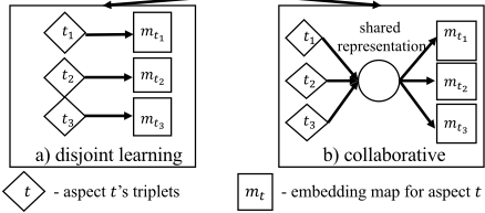
Fig. 1 outlines two approaches for conditional ordinal embedding problem (Eq. 1). The straightforward approach is disjoint learning, i.e., deriving a map for each aspect independently. Specifically, the map mt1 is learnt from only aspect t1's triplets, and the various maps mt1 to mt3 are not related (Fig. 1 left).
We believe that the aspects are potentially related as they concern the same set of objects. Their latent relationships could render significant advantage when aspects are sufficiently related, and yet each aspect is under-sampled. In practice, we do not necessarily observe all possible triplets, but a subset. For sparse data, an aspect may have insufficient information. Furthermore, the triplets of any one aspect may not cover all objects [Agarwal et al., 2007].
We propose a collaborative approach (Fig. 1 right). The challenge is to design a shared representation that allows "sharing" across aspects, and yet still allows each aspect to remain distinct. Here, we adopt a well-known instance of Riemannian manifold [Gilkey and others, 1975], namely: hypersphere. Every aspect has a coordinate on this shared hypersphere and its embedding is expressed on the hyperplane tangent at that aspect's coordinate. Every object also has a coordinate on this shared hypersphere. The projection of the objects' spherical coordinates onto the tangent hyperplane of a aspect constructs a map that reveals that aspect's distinct "point of view" or perception of similarity. We elaborate this modeling in the next section.
4 Spherical Conditional Ordinal Embedding
Each aspect t ∈ T and object i ∈ I are respectively associated with a spherical coordinate xt, yi ∈ SK , where SK = {p ∈ RK+1 : ||p|| = 1}. The output coordinate yt i ∈ RK is the projection of yi onto task-specific Kdimensional hyperplane defined by xt. The intuition for a sphere as the shared representation is that it allows greater flexibility for each aspect to model its own similarity perception, while still being embedded within the same hyperspace and sharing the same geometric shared representation.
4.1 Model
To arrive at shared Y = {yi : i ∈ I}, while accommodating variances among aspects, we turn to probabilistic modeling.
Generative Process
Let us first consider an individual conditional ordinal triplet 〈i, j, k〉t ∈ N. We associate an aspect t and three objects i, j, and k with a binary-valued random variable ctijk . When ctijk = 1, we generate the triplet 〈i, j, k〉t ∈ N, i.e., t considers j to be more similar to i than to k. If ctijk = 0, opposing triplet 〈k, j, i〉t ∈ N is generated.
There are two views of relative proximity, which determines the outcome of ctijk . First, there is the aspect-specific view of an aspect t, based on the projected coordinates on t's tangent hyperplane, for which the probability is Pt(ctijk = 1|yt i , yt j , ytk ). Second, there is the global view, based on coordinates on the shared sphere, for which the probability is Ps(ctijk = 1|yi, yj, yk). We assume that some triplets are aspect-specific, generated according to Pt, while other triplets are generic, generated according to Ps. The balance between the two is modeled by parameter δt ∈ [0, 1].
Now we describe the generative process for triplets in N:
- For each task t ∈ T :
- Draw t's coordinate: xt ∼ VMF (µT , κT )
- Draw t's parameter δt: δt ∼ U(0, 1)
- For each object i ∈ I:
- Draw i's coordinate: yi ∼ VMF (µI, κI)
- For objects i, j, k ∈ I, i < k, j ̸= i, k:
- If a draw fromBernoulli (δt) turns up 1, then: ctijk ∼ Bernoulli (Pt(ctijk = 1|yt i , yt j , ytk )) Else: ctijk ∼ Bernoulli (Ps(ctijk = 1|yi, yj , yk))
- If ctijk = 1, generate a triplet instance〈i, j, k〉t, Else: generate a triplet instance〈k, j, i〉t.
In the above generative process, xt and yi have von MisesFisher (vMF) [Mardia, 1975] priors, parameterized by mean unit vector µ and concentration κ. Higher κ translates to greater concentration around µ. κ = 0 models the uniform prior. In this paper, we assume that δt has a uniform prior.
Aspect-Specific Probability Function
Given the shared spherical representation, and the intention to maintain each aspect's embedding on a Euclidean space, a natural choice is to have the aspect-specific representation lie on the tangent hyperplane of sphere SK at xt, defined as: Txt SK = {v ∈ RK+1 : (xt)T v = 0}. We define the aspectspecific representation for t to be the projection of objects' coordinates {yi : i ∈ I} onto the tangent hyperplane at xt:
where I is (K +1)-dimensional identity matrix 1 .
1 Though Projxt (yi) is a (K + 1)-dimensional vector, it still effectively lies on a K-dimensional tangent hyperplane in the (K + 1)-dimensional space. In the appendix, we describe in detail the
K-dimensional coordinate transformation.
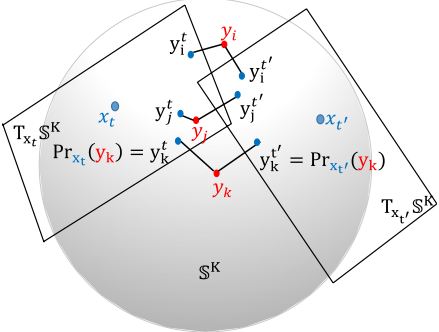
Fig.2 illustrates an example of the representations yi, yj , yk of three objects i, j, k (red points) and xt, xt′ of two aspects t, t′ (blue points) on the unit sphere. The left tangent hyperplane Txt S K corresponds to the representation map of aspect t. On this map, yt j is closer to ytk than to yt i through the projection Projxt . The right tangent hyperplane Txt′ S K is the representation map of aspect t′ . There, yt′ j is closer to yt′ i than to yt′ k . These are "conflicting" ordinal relationships between t and t′ , yet they arise from the same spherical coordinates of objects, indicating the role of aspects' tangent hyperplanes in accommodating different similarity perceptions. There are also triplets which both t and t′ agree on.
We now express Pt in terms of such projected distances. Let us denote the distance dtij between two objects i, j on aspect t's map, i.e., dtij = ||Projxt (yj - yi)||. We express Pt(ctijk = 1|yt i , yt j , ytk ) in terms of difference between dtjk and dtij (Eq. 3). The smaller is dtij relative to dtjk , the higher is this probability. α is the scaling factor.
Global Probability Function
We now describe the "global" probability Ps - the likelihood of observing the triple 〈i, j, k〉t based on the objects' spherical coordinates. On the unit sphere, the distance between yi and yj is the geodesic distance [Ferreira et al., 2014]: gd(yi, yj ) = cos-1 (yi T yj ).
Given yi, yj , yk ∈ SK , the following relation holds:
On one hand, Eq.4 implies that the inner product yields the same ordering as the geodesic distance. On the other hand, inner product computation is more computationally efficient compared to the geodesic distance. Therefore, the global probability is defined as follows:
Objective Function
The likelihood of observing the triplet 〈i, j, k〉t is the normalized weighted sum of Pt and Ps. The formula is described in Eq. 6 below.
The model's parameters are learnt to maximize the joint probability P(N,X, Y |κT , µT , κI, µI) of the model across the observed triplets (Eq. 7), which can be factorized as product of P(Nt|X, Y ) = ∏〈i,j,k〉t∈Nt lt ijk - the likelihood, and P(X|κT , µT ) and P(Y |κI, µI) - the priors.
Maximizing the joint probability in Eq. 7 is equivalent to maximizing its logarithm L (to simplify the parameters, we tie κT = κI = κ and µT = µI = µ):
4.2 Parameter Learning
Line Search on Manifold
The learning requires solving an optimization problem on the spherical manifold. [Absil et al., 2009] presents the linesearch method on a manifold M. The update formula is: xk+1 = Rxk (tkηk), - Rxk , tk, and ηk ∈ TxkM are the retraction map at xk, the step size, and the search direction respectively. Retraction map ensures the update process to be performed on the manifold. Here, we consider the following map [Bonnabel, 2013]:
For parameter learning, we adopt the stochastic gradient descent strategy for functions defined on a Riemannian manifold [Bonnabel, 2013], which requires the computation of the Riemannian gradient. According to [Ferreira et al., 2014], the gradient on the sphere of a differentiable function f : Ω → R (let Ω ∈ SK be an open set), at x ∈ Ω is defined by:
where ∇f(x) is the usual gradient of f(x) at x ∈ Ω.
Learning Algorithm
Algorithm 1 shows that in each iteration, a triplet 〈i, j, k〉t is randomly selected, and the parameters are updated using the line-search optimization technique on the unit sphere. Specifically, we first compute the partial derivatives with respect to xt, yi, yj, yk (line 7). The gradients on the spherical surface are computed through the project map Proj(.). Then we update the model parameters using the retraction map as described earlier (line 9). Learning rate ϵ is decayed over time. The last update in line 10 guarantees that δt ∈ [0, 1]. The complexity is linear to the size of N-the set of all triplets, which is bounded by O(|T | × |I|3 ).
Algorithm 1 SCORE
- 1: Initialize xt for t ∈ T and yi for i ∈ I.
- 2: While not converged
- 3: Draw a triplet 〈i, j, k〉t randomly fromN.
- 4: Compute the likelihood:
- 5: lt ijk = δt.σt ijk + (1 - δt)σijk.
- 6: Compute the partial derivatives:
- 7: ∆z ← ∂L ∂z for each z ∈ {xt, yi, yj, yk}
- 8: Update the model parameters:
- 9: z ←Rz (ϵ.Projz (∆z)), for z ∈ {xt, yi, yj, yk} ;
- 10: δt ← δt + ϵ. (σt ijk - σijk ) ; δt = arg min δ∈[0,1] |δt - δ|;
- 11: Return {xt}t∈T and {yi}i∈I.
5 Experiments
Our objective is primarily to investigate the effectiveness of multiple maps for conditional or dinal embedding.
5.1 Experimental Setup
Datasets
We experiment with three public datasets that could model varying perceptions of similarity.
- Zoo 2 contains 17 attributes of 101 animals (excluding animal name). We model each attribute as a similarity aspect. For attribute t, we form the triplet 〈i, j, k〉t if i and j have the same attribute value, which is different from k. There are 3.24 × 10⁶ triplets.
- Congressional Voting Records (or HouseVote) 3 contains 435 instances (congressmen) and 16 attributes (voting issues). After excluding instances with missing values, we get 232 fully-observed instances of 16 attributes. We generate triplets in the same way as we do with Zoo dataset. That induces totally 2.4×10⁷ triplets.
- Paris Attractions 4 contains 237 users organizing 250 Paris attractions into clusters. With user as aspect, we induce 3.48×10⁵ triplets, each involves two attractions i and j that the user puts into the same cluster, and another attraction k in a different cluster. As in [Yue et al., 2014], we exclude attractions uninteresting to users.
Comparative Methods
We compare SCORE to several baselines. The disjoint learning approach (Section 3) learns a distinct map from the triplets of an aspect. We use two recent ordinal embedding methods: SOE 5 [Terada and Luxburg, 2014] and tSTE 6 [Van der Maaten and Weinberger, 2012].
Multiview Triplet Embedding (MVTE) [Amid and Ukkonen, 2015] divides one pool of triplets into clusters. The number of views is set to the number of aspects, i.e., |T |. Since the aspect-triplet associations are unknown, we match each view with a ground-truth attribute using Hungarian maximum bipartite matching algorithm, so as to maximize the accuracy.
2 https://archive.ics.uci.edu/ml/datasets/Zoo
3 https://archive.ics.uci.edu/ml/datasets/congressional+voting+records
4 http://projects.yisongyue.com/collab_cluster/
5 https://rdrr.io/cran/loe/
6 https://lvdmaaten.github.io/ste/Stochastic_Triplet_Embedding
Multiview Multidimensional Scaling (MVMDS) [Bai et al., 2017] performs MDS on multi-view data, learns the weights of these views, and produces one consensus map. This is akin to learning a single map by consolidating multiple views. Since MVMDS expects distance matrices, we feed it feature vectors learnt by SOE from the ordinal triplets.
For visualization purpose, we set the dimensionality of the embedding space K = 2. We tune the parameters of all methods for their best performances on the training data. For SCORE, the setting is κ = 10-3 for Paris Attractions, and 0 for Zoo and HouseVote, vMF mean vector µ = (0, 0, 1), the learning rate ϵ = 0.05, and the scaling factor α = 30. For SOE, the scaling factor is 0.1 for all the datasets. For tSTE, the learning rate and regularization parameter are 2 and 0 respectively for all datasets. For MVTE, the learning rate is 1 for all datasets. For MVMDS, γ = 5 for all datasets.
Evaluation Measure
The preservation accuracy for an aspect t is the fraction of its ordinal triplets Nt for which t's coordinates reflect the correct direction. The fewer the violated triplets, the higher is the accuracy. The overall accuracy is the average of aspects' preservation accuracies (Eq. 10):
- yt i , yt j , ytk are t's embedding coordinates of objects i, j, k. Since in practice we may not observe all triplets or even all objects beforehand, we sample a fraction r (split ratio) of objects for each aspect, then evaluate the coordinates against the full set of triplets. As the default for this study, we set r = 0.5, which has a relative balance between the information that an aspect sees and the information that it could learn from others. Later we will also investigate the effects of different r values. We average the results across 30 random samples.
The running times are reasonable. For the Paris Attractions, including all aspects, SCORE takes 5 minutes on a PC with Intel Core i5 3.2 GHz CPU and 12 GB RAM. The learning times for the Zoo and HouseVote are less than 10 minutes.
5.2 Comparison to Baselines
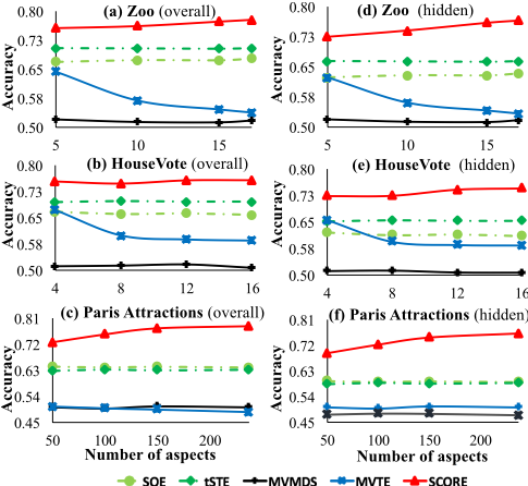
We vary the number of aspects by randomly sampling aspects. Fig. 3 shows the preservation accuracies of all models.
Overall Preservation Accuracy
SCORE shows significantly higher performance than SOE, tSTE (Fig. 3(a,b,c)). In the latter, an aspect cannot collaborate with other aspects, leading to poor performance on unseen triplets. This highlights the benefit of collaborative learning, as it helps aspects fill in each other's missing information. MVTE and MVMDS show even weaker performances. For MVTE, the likely reason is the lack of information about the associations between aspects and triplets. If this information is provided, MVTE reduces to tSTE, which is showing relatively higher performance than MVTE. For MVMDS, the likely reason is the consolidation into a single map, which, though learnt from multiple distance matrices, cannot fit conflicting triplets.
Performance on Predicting Hidden Triplets
The earlier accuracies are evaluated for the full set of triplets, which is the combination of the observed subset (from the r fraction) and the hidden subset (the unseen triplets). To see how well the models generalize to the unseen data, we now investigate the preservation accuracy measured on the hidden alone (Fig. 3(d,e,f)). We observe the same picture as before but with generally lower accuracies than that for full sets (Fig. 3(a,b,c)), which are expected as these are unseen triplets. The reduction is more dramatic for SOE and tSTE, which tend to overfit the observed, and generalize poorly to the hidden triplets. SCORE does commendably well on the hidden set, showing greater robustness in generalizing to the unseen triplets.
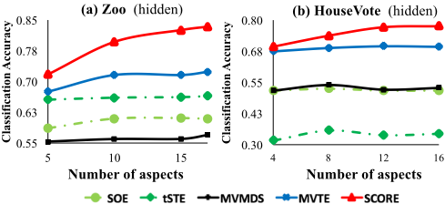
For an alternative measure of generalization, we test the learnt coordinates as features to classify the hidden objects by attribute values associated with the aspect. An object is assigned the majority label among its 10-nearest neighbors. Fig. 4 shows the 10-NN classification accuracy, averaged across aspects. Only Zoo and HouseVote have "labels" and are involved in this experiment. SCORE has better results than the baselines (statistically significant at 0.05) in predicting the labels of unseen instances. Interestingly, MVTE performs better than disjoint learning baselines in this task. Since triplets are learned jointly, some triplets may have been assigned to clusters correlated with the class labels, though the clusters may not reflect the aspect-specific view perfectly.
Exploration on the Split Ratio
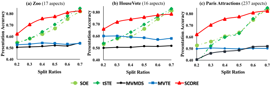
To better understand the benefits of multi-aspect modeling, we shows the accuracies with varying r for the complete set of aspects in Fig. 5.
The disjoint learning baselines perform poorly for low value of r. This is expected since the amount of observed data is insufficient for a single task to learn its own map effectively. For extremely high r, e.g., 0.7, the disjoint learning baselines tend to do well. For Zoo, HouseVote, and Paris Attractions, r = 0.7 respectively corresponds to approximately 1.1M, 16.1M, and 155K triplets in training, which are 34.23%, 34.17%, and 44.42% of all possible triplets. With sufficiently large data that cover majority of objects, each aspect has more flexibility to specialize, with little risk in missing out information. Also in Fig. 5, SCORE shows significantly better performances than MVTE and MVMDS for the same reasons that have been discussed in the first experiment.
Importantly, SCORE is robust across values of r. It is the best around 0.2-0.6, and never the worst. This result has two implications. First, it reiterates the benefit of collaborative approach when the data is under-sampled, yet sufficient to learn the relatedness and specialization of tasks. Second, in practice it is often unclear whether the data is sufficient. Upon such ambiguity, multi-aspect modeling ameliorates the risk of performing badly, while providing reasonable performance.
5.3 Aspect Relatedness
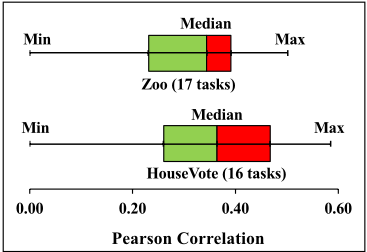
Two similar aspects would be expected to be closer on the hypersphere than two dissimilar aspects. For Zoo and HouseVote, each aspect corresponds to an attribute, whose values effectively define a clustering of objects. We define the attribute-based similarity between two aspects as the Normalized Mutual Information or NMI [Estévez et al., 2009] between the two clusterings. We also define the proximity between two aspects on the shared hypersphere as their angular similarity. For each aspect t ∈ T , we measure the Pearson correlation of the NMI scores and angular similarities between t and other aspects in T . We observe positive correlations among the NMI scores and the angular similarities (Fig. 6). The minimum values for both datasets are non-negative and the median values are quite positive 0.34 and 0.36 for Zoo and HouseVote respectively, indicating that SCORE captures aspect relatedness during learning, with similar aspects more likely to be closer on the hypersphere.
5.4 Multiple Maps vs. Single Map
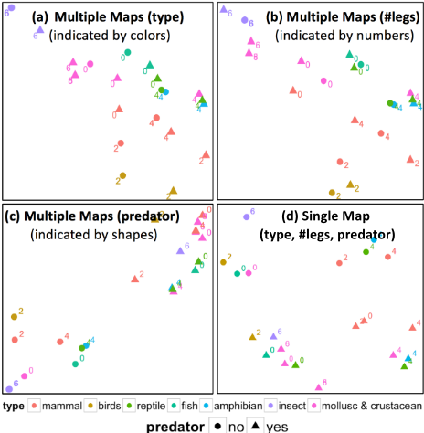
To better illustrate the need for multiple maps, we consider a scenario involving three attributes of a dataset (type, #legs, predator from Zoo, and immigration, education-spending, crime from HouseVote). We compare SCORE in two modes: multiple maps when we learns three distinct maps collaboratively and single map when we pool triplets from the three attributes to learn one map. Table 1 compares the preservation accuracies of the two modes, showing that multiple maps have significally higher accuracies, indicating its greater capacity for reflecting multiple aspects than a single map.
As a visual illustration, Fig.7(a, b, c) shows the three maps (corresponding to multiple maps) concerning animals from Zoo. Each animal is shown as a point, whose color, number, and shape indicate type, #legs, and predator attributes respectively. Fig. 7(a) visualizes animals based on type (color). Animals of the same type (color) flock together, e.g., insects (purple) on the top left, birds (yellow) on the bottom right. Fig. 7(b) visualizes animals in terms of #legs. Animals of the same number of legs tend to be found together, e.g., 6 legs on the top left, 2 legs on the bottom right. Fig. 7(c) visualizes animals based on whether they are predator (shape). The binary separation of predators (triangles) on the top right and nonpredators (circles) on the lower left is evident. A single map cannot capture diverse perceptions of similarity. Fig. 7(d) depicts the single map mode for the same three attributes. It could only represent separation by predator (shape), but is unable to represent type or #legs well.
| SCORE | Zoo | HouseVote |
|---|---|---|
| Single Map | 0.82 | 0.70 |
| Multiple Maps | 0.98 | 0.89 |
6 Conclusion
In this work, we formulate the problem of ordinal embedding involving ordinal comparisons from multiple aspects as conditional ordinal embedding. Our proposed geometric approach seeks to represent aspects and objects on a shared hypersphere, as well as on aspect-specific tangent hyperplanes. Experiments on public datasets show that the proposed framework is robust, and particularly beneficial when there is variance across tasks yet insufficient data to learn each task separately, thus collaboration across tasks is helpful.
Acknowledgements
This research is supported by the National Research Foundation, Prime Minister's Office, Singapore under its NRF Fellowship Programme (Award No. NRF-NRFF2016-07).
A K-dimensional Coordinate Transformation
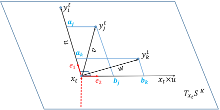
A necessary step is to transform the (K + 1)-dimensional coordinate of objects on t's tangent hyperplane, i.e., {Projxt (yi)}i∈I, to their corresponding K-dimensional coordinates, i.e., {yt i }i∈I. For the purpose of visualizing the embedding for an aspect t on a scatterplot, we describe how to transform the 3D coordinates of objects on t's tangent hyperplaneto their corresponding 2D coordinates in the following. However, the below analysis is also applicable to highdimensional embedding space, i.e., when K > 2.
Since xt,Projxt (yi),Projxt (yj), Projxt (yk) lie on the tangent hyperplane Txt SK of the task t, the three vectors: u = Projxt (yi)-xt; v = Projxt (yj )-xt; w = Projxt (yk)- xt are on Txt SK as well.
As illustrated in Fig. 8, the cross product xt ×u is a vector on Txt SK and perpendicular to xt, u. Let's denote:
We can see that e1, e2 form a basis of Txt SK (since ||e1|| = ||e2|| = 1, e1 T e2 = 0). From linear algebra, for each point y ∈ Txt SK , there exists unique ay, by ∈ R such as:
Consider the following transformation map where ay, by ∈ R are defined as above:
Let (aj, bj) and (ak, bk) be the transformation of Projxt (yj) and Projxt (yk) respectively:
Equation 12 implies that the L2-norm between points on Txt SK are preserved through the transformation map Trt. Therefore, the ordinal relations between points are also preserved through the transformation. Hence, we express yt i = Trt(Projxt (yi)), for all i ∈ I.
@inproceedings{ijcai2019p390,
  title     = {Learning Multiple Maps from Conditional Ordinal Triplets},
  author    = {Le, Dung D. and Lauw, Hady W.},
  booktitle = {Proceedings of the Twenty-Eighth International Joint Conference on
               Artificial Intelligence, {IJCAI-19}},
  publisher = {International Joint Conferences on Artificial Intelligence Organization},
  editor    = {Sarit Kraus},
  pages     = {2815--2822},
  year      = {2019},
  month     = {8},
  note      = {Main track},
  doi       = {10.24963/ijcai.2019/390},
  url       = {https://doi.org/10.24963/ijcai.2019/390},
}
TY - CPAPER TI - Learning Multiple Maps from Conditional Ordinal Triplets AU - Le, Dung D. AU - Lauw, Hady W. T2 - Proceedings of the Twenty-Eighth International Joint Conference on Artificial Intelligence, IJCAI-19 PB - International Joint Conferences on Artificial Intelligence Organization PY - 2019 SP - 2815 EP - 2822 DO - 10.24963/ijcai.2019/390 UR - https://doi.org/10.24963/ijcai.2019/390 ER -Copied
Machine-readable versions of this paper, for tools and AI agents:





