
Flexible Multi-View Representation Learning for Subspace Clustering
Proceedings of the Twenty-Eighth International Joint Conference on Artificial Intelligence. Main track. Pages 2916-2922.
https://doi.org/10.24963/ijcai.2019/404
Keywords
- Machine Learning: Multi-instance;Multi-label;Multi-view learning
- Machine Learning: Clustering
Abstract
In recent years, numerous multi-view subspace clustering methods have been proposed to exploit the complementary information from multiple views. Most of them perform data reconstruction within each single view, which makes the subspace representation unpromising and thus can not well identify the underlying relationships among data. In this paper, we propose to conduct subspace clustering based on Flexible Multi-view Representation (FMR) learning, which avoids using partial information for data reconstruction. The latent representation is flexibly constructed by enforcing it to be close to different views, which implicitly makes it more comprehensive and well-adapted to subspace clustering. With the introduction of kernel dependence measure, the latent representation can flexibly encode complementary information from different views and explore nonlinear, high-order correlations among these views. We employ the Alternating Direction Minimization (ADM) method to solve our problem. Empirical studies on real-world datasets show that our method achieves superior clustering performance over other state-of-the-art methods.
- [Amini et al., 2009] Massih-Reza Amini, Nicolas Usunier, and Cyril Goutte. Learning from multiple partially ob- served views -an application to multilingual text catego- rization. In NIPS, pages 28-36, 2009.
- [Andrew et al., 2013] Galen Andrew, Raman Arora, Jeff A. Bilmes, and Karen Livescu. Deep canonical correlation analysis. In ICML, pages 1247-1255, 2013.
- [Bach and Jordan., 2002] Francis R. Bach and Michael I. Jordan. Kernel independent component analysis. In JMLR, pages 1-48, 2002.
- [Cai et al., 2010] Jian-Feng Cai, Emmanuel J. Candès, and Zuowei Shen. A singular value thresholding algorithm for matrix completion. Siam Journal on Optimization, 20(4):1956-1982, 2010.
- [Cao et al., 2015] Xiaochun Cao, Changqing Zhang, Huazhu Fu, Si Liu, and Hua Zhang. Diversity-induced multi-view subspace clustering. In CVPR, pages 586-594, 2015.
- [Chaudhuri et al., 2009] Kamalika Chaudhuri, Sham M. Kakade, Karen Livescu, and Karthik Sridharan. Multi- view clustering via canonical correlation analysis. In ICML, pages 129-136, 2009.
- [De Sa, 2005] Virginia R. De Sa. Spectral clustering with two views. In ICML, pages 20-27, 2005.
- [Elhamifar and Vidal, 2013] Ehsan Elhamifar and Rene Vi- dal. Sparse subspace clustering: Algorithm, theory, and applications. IEEE TPAMI, 35(11):2765-2781, 2013.
- [Gao et al., 2013] Jing Gao, Jiawei Han, Jialu Liu, and Chi Wang. Multi-view clustering via joint nonnegative matrix factorization. In ICDM, pages 252-260, 2013.
- [Gretton et al., 2005] Arthur Gretton, Olivier Bousquet, Alexander J. Smola, and Bernhard Schölkopf. Measur- ing statistical dependence with hilbert-schmidt norms. In Proceedings of the international conference on Algorith- mic Learning Theory, pages 63-77, 2005.
- [Hotelling, 1936] Harold Hotelling. Relations between two sets of variates. Biometrika, 28(3/4):321-377, 1936.
- [Hu et al., 2014] Han Hu, Zhouchen Lin, Jianjiang Feng, and Jie Zhou. Smooth representation clustering. In CVPR, pages 3834-3841, 2014.
- [Kumar et al., 2011] Abhishek Kumar, Piyush Rai, and Hal Daume. Co-regularized multi-view spectral clustering. In NIPS, pages 1413-1421, 2011.
- [Lampert et al., 2014] Christoph H Lampert, Nickisch Hannes, and Harmeling Stefan. Attribute-based classifi- cation for zero-shot visual object categorization. IEEE TPAMI, 36(3):453-465, 2014.
- [Lin et al., 2011] Zhouchen Lin, Risheng Liu, and Zhixun Su. Linearized alternating direction method with adap- tive penalty for low-rank representation. In NIPS, pages 612-620, 2011.
- [Liu and Yan, 2011] Guangcan Liu and Shuicheng Yan. La- tent low-rank representation for subspace segmentation and feature extraction. In ICCV, pages 1615-1622, 2011.
- [Liu et al., 2013] Guangcan Liu, Zhouchen Lin, Shuicheng Yan, Ju Sun, Yong Yu, and Yi Ma. Robust recovery of sub- space structures by low-rank representation. IEEE TPAMI, 35(1):171-184, 2013.
- [Lu et al., 2012] Can-Yi Lu, Hai Min, Zhong-Qiu Zhao, Lin Zhu, De-Shuang Huang, and Shuicheng Yan. Robust and efficient subspace segmentation via least squares regres- sion. In ECCV, pages 347-360, 2012.
- [Luo et al., 2011] Dijun Luo, Feiping Nie, Chris Ding, and Heng Huang. Multi-subspace representation and discov- ery. In ECML-PKDD, 2011.
- [Ng et al., 2001] Andrew Y. Ng, Michael I. Jordan, and Yair Weiss. On spectral clustering: Analysis and an algorithm. In NIPS, pages 849-856, 2001.
- [Patel et al., 2013] Vishal M. Patel, Hien Van Nguyen, and René Vidal. Latent space sparse subspace clustering. In ICCV, pages 225-232, 2013.
- [Tao et al., 2017] Zhiqiang Tao, Hongfu Liu, Sheng Li, Zhengming Ding, and Yun Fu. From ensemble clustering to multi-view clustering. In IJCAI, 2017. IJCAI
- [Tao et al., 2019] Zhiqiang Tao, Hongfu Liu, Sheng Li, Zhengming Ding, and Yun Fu. Marginalized multiview ensemble clustering. IEEE TNNLS, pages 1-12, 2019.
- [Wang et al., 2007] Meng Wang, Xian-Sheng Hua, Xun Yuan, Yan Song, and Li-Rong Dai. Optimizing multi- graph learning: towards a unified video annotation scheme. In ACM Multimedia, pages 862-871, 2007.
- [Wang et al., 2017] Xiaobo Wang, Xiaojie Guo, Zhen Lei, Changqing Zhang, and Stan Z. Li. Exclusivity-consistency regularized multi-view subspace clustering. In CVPR, pages 1-9, 2017.
- [Wei et al., 2009] Tang Wei, Zhengdong Lu, and Inderjit S. Dhillon. Clustering with multiple graphs. In ICDM, pages 1016-1021, 2009.
- [White et al., 2012] Martha White, Xinhua Zhang, Dale Schuurmans, and Yao liang Yu. Convex multi-view sub- space learning. In NIPS, pages 1673-1681, 2012.
- [Wu et al., 2013] Baoyuan Wu, Yifan Zhang, Bao-Gang Hu, and Qiang Ji. Constrained clustering and its application to face clustering in videos. In CVPR, pages 3507-3514, 2013.
- [Xia et al., 2014] Rongkai Xia, Yan Pan, Lei Du, and Jian Yin. Robust multi-view spectral clustering via low-rank and sparse decomposition. In AAAI, 2014.
- [Xu et al., 2016] Jinglin Xu, Junwei Han, and Feiping Nie. Discriminatively embedded k-means for multi-view clus- tering. In CVPR, pages 5356-5364, 2016.
- [Zhang et al., 2015] Changqing Zhang, Huazhu Fu, Liu Si, Guangcan Liu, and Xiaochun Cao. Low-rank tensor con- strained multiview subspace clustering. In ICCV, pages 1582-1590, 2015.
- [Zhang et al., 2017] Changqing Zhang, Qinghua Hu, Huazhu Fu, Pengfei Zhu, and Xiaochun Cao. La- tent multi-view subspace clustering. In CVPR, pages 4279-4287, 2017.
References were extracted automatically from the PDF and may contain errors.
Full text extracted automatically from the PDF; figures, tables and equations may differ. The PDF is the version of record.
1 Introduction
Subspace clustering is a fundamental method for recovering the subspace structure of data, especially for highdimensional data. Recently, self-representation-based subspace clustering methods [Elhamifar and Vidal, 2013; Liu et al., 2013; Hu et al., 2014] have been proposed, which are based on the assumption that each data point can be reconstructed using the dictionary formed by all data points. Sparse Subspace Clustering (SSC) [Elhamifar and Vidal, 2013] clusters data based on sparse representation which can be obtained by ℓ1-norm. Low-Rank Representation (LRR) [Liu et al., 2013] aims to search for a lowest-rank representation among all the candidates. Smooth Representation clustering (SMR) [Hu et al., 2014] introduces the grouping effect for subspace clustering. The above mentioned methods have produced promising performances, however, they only focus on boosting single-view clustering.
In many real-world applications, data are often from multiple sources. For example, a document might be described by images, video, text, and audio. Human activities may be captured by video cameras, depth cameras, and on-body sensors. These different views often contain complementary information to each other, hence exploiting the complementarity among multiple views could potentially advance the clustering performance.
Considering that each individual view is insufficient for depicting data points, recently, subspace clustering has been extended to multi-view cases [Cao et al., 2015; Zhang et al., 2015; Zhang et al., 2017]. With the introduction of low-rank tensor constraint or exploration of the diversity among different subspace representations, LT-MSC [Zhang et al., 2015] and DiMSC [Cao et al., 2015] could well explore complementary information from multiple sources and improve the subspace clustering by a large margin. However, there are two main limitations in these approaches: (1) they reconstruct data within each single view using original noisy features, which is insufficient to describe data; (2) they only exploit linear subspaces of data in the raw feature space, which is not enough for capturing complex correlations among real-world data.
One important technique for identifying the relationships among different views and simultaneously constructing a common space is Canonical Correlation Analysis (CCA) [Chaudhuri et al., 2009]. Although simple, CCA-based methods have the following limitations: (1) they project multiple views into a common space by improving their correlations, but cannot well address the complementarity of different views; (2) the dimensionalities of different views are reduced to the same, which is not suitable for the cases when the dimensionalities of two views are extremely unbalanced; (3) multi-view common representation learning process is separated from subspace clustering, which will cause the common representation not well-adapted to subspace clustering.
To address above issues, we propose a novel Flexible Multi-view Representation (FMR) learning method to construct a latent representation. Differing from CCA, we adopt the kernel dependence measure to drive the latent representation closely correlated to each view, so that there is no need to project multiple views into a common space. By mapping original features into the kernel space, the high-order and nonlinear dependence among different views can be captured.
The latent representation effectively facilitates subspace clustering, and meanwhile its comprehensiveness is promoted by subspace reconstruction. The main contributions of this paper include:
- We propose to conduct subspace clustering based on Flexible Multi-view Representation (FMR) learning, which avoids using partial information for data reconstruction and makes the latent representation welladapted to subspace clustering.
- We propose to construct a latent representation by encouraging it to be similar to different views in a weighted way, which implicitly enforces it to encode complementary information from multiple views.
- We introduce the kernel dependence measure: Hilbert Schmidt Independence Criterion (HSIC), to capture high-order, non-linear relationships among different views, which benefits recovering underlying cluster structure of data.
- Our model can be efficiently optimized by the Alternating Direction Minimization (ADM) method. Extensive experiments on benchmark datasets show its effectiveness.
2 RelatedWork
For single-view subspace clustering methods, the major difference lies in the constraint on subspace representation. LRR [Liu et al., 2013] and SSC [Elhamifar and Vidal, 2013] encourage subspace representations to be low-rank and sparse, respectively. Multi-Subspace Representation (MSR) [Luo et al., 2011] combines both criteria of LRR and SSC. Least Squares Regression (LSR) [Lu et al., 2012] improves grouping effect of data by Frobenius norm. Recently, researchers propose some subspace clustering methods based on latent space [Liu and Yan, 2011; Patel et al., 2013]. Latent Space Sparse Subspace Clustering (LS3C) [Patel et al., 2013] integrates dimensionality reduction and subspace clustering into a unified framework. Latent Low-Rank Representation (LatLRR) [Liu and Yan, 2011] is an enhanced version of LRR, which constructs the dictionary using both observed and unobserved data. Above mentioned methods implement subspace clustering in the single view without considering the multi-view cases.
With the growing amount of data from multiple sources, multi-view clustering has been widely studied and applied in real-world applications. De Sa proposes to create a bipartite graph and performs spectral clustering based on "minimizingdisagreement" idea [De Sa, 2005]. Multi-view clustering via Canonical Correlation Analysis (CCA) [Chaudhuri et al., 2009] projects different views into a common lowdimensional space. Some approaches [Wei et al., 2009; Gao et al., 2013] employ matrix factorization technique for multi-view clustering. Gao et al. address large-scale issue under the K-means framework [Gao et al., 2013]. The co-regularized method [Kumar et al., 2011] searches for a consistent clustering result across different views with a coregularization constraint. The convex representation learning method [White et al., 2012] enforces the conditional independence among separate views and simultaneously reduces the dimensionality. Tao et al. conduct multi-view clustering in an ensemble clustering way, which constructs a consensus partition of data across different view-specific basic partitions [Tao et al., 2017; Tao et al., 2019]. Robust Multiview Spectral Clustering [Xia et al., 2014] recovers a shared low-rank transition probability matrix as an input to the standard Markov chain. The recently proposed subspace methods [Cao et al., 2015; Zhang et al., 2015; Zhang et al., 2017; Wang et al., 2017] incorporate multi-view information under the self-representation-based subspace clustering framework.
Different from linear cases, we further explore the highorder, nonlinear relationships among different original views, so that the latent representation could properly depict data and reveal the intrinsic cluster structure shared by multiple views.
3 Proposed Approach
3.1 Subspace Clustering
Self-representative subspace clustering is quite effective for high-dimensional data. Suppose X=[x1, x2, ..., xN] ∈ Rd×N is the sample matrix, each column of which represents a data point, d is the dimensionality of feature space and N is the number of samples. To cluster data into their respective subspaces, we infer an coefficient matrix Z that reflects the similarity among data points. Without loss of generality, the formulation of subspace clustering can be written as:
where L(·, ·) and Ω(·) are loss function associated with data reconstruction and regularization term respectively, and the scalar λ > 0 is used to balance these two terms. Based on the coefficient matrix Z, the similarity matrix S is further obtained by S = abs(Z) + abs(ZT ), where abs(·) is the element-wise absolute operator. Then it is taken as an input for spectral clustering algorithm [Ng et al., 2001] to produce the final results.
Although above methods have achieved promising performances, they tend to be affected by original features, especially when each single view is insufficient to depict data.
3.2 Measuring Dependence
In this work, we propose a novel method to flexibly learn a common latent representation H by maximizing the dependence between it and different views. In this paper, we adopt the Hilbert-Schmidt Independence Criterion (HSIC) to measure dependence in the kernel space. The basic idea is to map original views into the Reproducing Kernel Hilbert Spaces (RKHSs) to capture high-order, nonlinear dependence among different original features. Suppose that data points x and y are drawn from two feature spaces X and Y, respectively. φ(x) represents a mapping from x ∈ X to kernel space F. Similarly, ϕ(y) is a mapping from y ∈ Y to the other kernel space G. The linear cross-covariance operator Cxy is defined as:
where µx and µy are mean values of φ(x) and ϕ(y), respectively. ⊗ is the tensor product. Based on the cross-covariance operator, we have the following definition of HSIC:
Definition 3.1 [Gretton et al., 2005] Given separable RKHSs F, G and a joint distribution pxy, we define HSIC as the squared Hilbert-Schmidt norm of Cxy:
Given N independent observations drawn from the joint distribution pxy: {(x1, y1), ..., (xN , yN )} ⊆ X ×Y, denoted as X, Y, the empirical HSIC measure is defined as:
where Kx, Ky ∈ RN×N are Gram matrices with (Kx)ij = kx(xi, xj) =< φ(xi), φ(xj) >, (Ky)ij = ky(yi, yj) =< ϕ(yi), ϕ(yj) >, and where (L)ij = δij -N -1 centers the Gram matrices to have zero mean in the feature space, δij denotes the entity of identity matrix.
3.3 Formulation
Given N observations from V views, we denote the vth view of data as X(v) = {x(v) 1 , ..., x(v) N } ∈ Rdv×N , 1 ≤ v ≤ V . For exploring complementary information from different views, we employ HSIC as a measure of dependence to drive the latent representation H to be close to different views. Furthermore, considering the varying quality of different views, we give weight αγ v for the vth view, which encodes the degree of similarity between the vth view and the latent representation. γ is the parameter to adjust the weight distribution of different views [Wang et al., 2007]. That is to say, the view strongly correlated to H will be assigned large weight. Over all, the objective function to infer the latent representation is:
The latent representation is more comprehensive than any single view due to the encoded complementary information. We conduct subspace clustering on it and obtain the total objective function as follows:
The first term is used to integrate complementary information from multiple views into a latent representation. || · ||∗ denotes the nuclear norm, which enforces the subspace representation Z to be low-rank. We impose ℓ2,1-norm on reconstruction error E with ||E||2,1 = ∑Nj=1 √∑Ni=1 ([E]ij )2 to encourage columns of E to be zero [Liu et al., 2013]. The hyper-parameters λ1 and λ2 control the trade-off among the three terms.
4 Optimization
To make the objective function separable, we introduce an auxiliary variable J to replace Z, then Eq. (6) is converted to the following equivalent problem:
Accordingly, we solve the above problem by the Augmented Lagrange Multiplier (ALM) method, and induce the following objective function:
For convenience, we give the definition Φ(Y,C) = µ2 ||C||2F + 〈Y, C〉, where 〈·, ·〉 defines the matrix inner product, Y is Lagrange multiplier matrix, and µ is a positive penalty scalar. According to the LADMAP [Lin et al., 2011], Eq. (8) can be separated into the following subproblems:
H-subproblem. Fixing the other variables, we firstly update H by solving the following subproblem:
We optimize Eq. (9) with Gradient Descent algorithm (GD), where the gradient with respect to H is:
Z-subproblem. Fixing the other variables, we update Z by solving the following problem:
Taking the derivative with respect to Z and setting it to zero, we can update Z with the following rule:
E-subproblem. For updating the reconstruction error E, we solve the following problem:
The above subproblem can be solved by Lemma 4.1 in [Liu et al., 2013].
J-subproblem. The Lagrange function with respect to J can be optimized by:
This step can be solved by the Singular Value Thresholding (SVT) operator [Cai et al., 2010].
Algorithm 1: Optimization of our method
Input: Multi-view data: {X(1) , ...,X(V ) }, the number of clusters m, hyper-parameters λ1 and λ2, the dimensionality of latent representation K, and the parameter γ.
Initialize: E = 0, Z = J = 0, Y1 = 0, Y2 = 0, µ = 10-5 , ρ = 1.1, ε = 10-4 , maxµ = 1010 ; Initialize the latent representation Hwith random values and initialize the weight α = 1/V for all the views.
while not converged do
Update variables H, Z, E, J according to Eq. (10), (12)
-(14), respectively;
Update weight αv (1 ≤ v ≤ V ) according to Eq. (18); Update multipliers Y1,Y2 and penalty parameter µ according to Eq. (19);
Check the convergence conditions:
end
Output: H, Z, {α1,...,αV }.
Updating weights. αv (1 ≤ v ≤ V ): To update αv, we rewrite Eq. (7) as:
where
The Lagrange function of Eq. (15) is:
where β is the Lagrange multiplier. We set the derivative with respect to αv to zero, then we get:
Updating multipliers. Finally, the Lagrange multipliers Y1,Y2 and penalty parameter µ are updated according to LADMAP [Lin et al., 2011] algorithm:
where ρ is a positive scalar.
4.1 Complexity Analysis
The main complexities of self-representative subspace clustering methods (DiMSC [Cao et al., 2015], LT-MSC [Zhang et al., 2015], LMSC [Zhang et al., 2017]) are from the graph (with the size N ×N) involved, which leads to the computational cost of matrix operations (e.g., SVD decomposition and matrix inversion). There are two main steps for these methods, i.e., affinity matrix learning (step1) and spectral clustering (step2). We list the complexity of each step in Table 1. In general, the total complexities for all these methods on largescale data are O(N 3 ).
| Methods | Step 1 | Step 2 | Total |
|---|---|---|---|
| DiMSC | O(T V N 3 + V DN 2 ) | O(N 3 ) | O(N 3 ) |
| LT-MSC | O(T V N 3 + T V DN 2 ) | O(N 3 ) | O(N 3 ) |
| LMSC | O(T(D3 +N 3 +DKN +KN 2 )) | O(N 3 ) | O(N 3 ) |
| Ours | O(T (L + 1)(N 3 + KN 2 )) | O(N 3 ) | O(N 3 ) |
Table 1: Complexity analysis of different methods
5 Experiments
We conduct experiments on 7 datasets from different applications: images, text, and community networks.
- Yale 1 consists of 165 grayscale images of 15 individuals, from which 3 types of features are extracted.
- MSRC-v1 [Xu et al., 2016] consists of 210 images of 7 object classes, which includes 6 types of features.
- Notting-Hill [Wu et al., 2013] is a video face dataset consisting of 550 images of 5 main casts described from 3 different views. It is more challenging because of the rich facial expressions, changing angles, and varied light intensities.
- Reuters [Amini et al., 2009] is a multilingual dataset including 2000 newswire articles of 6 classes written in 5 languages (views).
- BBCSport 2 is composed of news articles in 5 topical areas from BBC website, which is associated with 2 views.
- Football 3 contains 248 English Premier League football players and clubs active on Twitter, which are described from 9 different views and associated with 20 clubs.
- ANIMAL [Lampert et al., 2014] contains 30475 images of 50 animal classes including 2 types of feature. 10158 samples are selected with fixed interval to generate a subset.
5.1 ComparedMethods
We compare our approach with 8 state-of-the-art baselines. SPCBestSV [Ng et al., 2001] performs standard spectral clustering within the best single view. Min-D [De Sa, 2005] creates a bipartite graph to minimize the disagreement between two views. Co-Reg SPC [Kumar et al., 2011] coregularizes the clustering hypotheses to be consistent across multiple views. RMSC [Xia et al., 2014] constructs a joint low-rank transition probability matrix as an input for spectral clustering. DiMSC [Cao et al., 2015] explores the diversity among subspaces of all views through kernel technique. LTMSC [Zhang et al., 2015] employs low-rank tensor to capture high-order relationships among different views. LMSC [Zhang et al., 2017] constructs an underlying latent representation through linear mapping and then conducts subspace clustering on it. ECMSC [Wang et al., 2017] simultaneously explores the representation complementarity and indicator consistency among different views.
1 http://cvc.yale.edu/projects/yalefaces/yalefaces.html
2 http://mlg.ucd.ie/datasets/
3 http://mlg.ucd.ie/aggregation/
| Datasets | Metrics | SPCBestSV | Min-D | Co-Reg | RMSC | DiMSC | LT-MSC | LMSC | ECMSC | FMR |
|---|---|---|---|---|---|---|---|---|---|---|
| Yale | NMI | 65.42±1.05 | 64.53±2.48 | 64.87±1.24 | 68.49±3.32 | 72.73±1.26 | 76.53±0.82 | 68.31±2.67 | 77.34±1.06 | 84.11±2.95 |
| ACC | 70.73±3.04 | 61.57±4.30 | 69.72±2.05 | 64.20±3.65 | 70.95±3.56 | 74.08±0.24 | 64.73±2.52 | 77.18±1.42 | 85.31±3.80 | |
| F-score | 47.52±1.12 | 47.06±0.59 | 46.63±3.04 | 51.74±4.31 | 56.38±2.34 | 59.83±0.62 | 51.81±2.19 | 61.70±1.25 | 72.17±4.57 | |
| RI | 92.99±0.65 | 92.68±0.34 | 92.64±0.50 | 93.36±0.87 | 93.64±0.41 | 94.17±0.08 | 93.92±0.27 | 94.62±0.51 | 95.23±0.64 | |
| MSRC-v1 | NMI | 57.42±3.16 | 60.64±0.35 | 56.92±1.25 | 58.57±0.56 | 62.87±2.18 | 70.04±0.13 | 65.34±0.15 | 66.86±0.44 | 71.68±1.51 |
| ACC | 66.82±4.26 | 69.21±3.45 | 65.30±1.65 | 69.10±0.71 | 68.57±3.92 | 80.00±0.09 | 80.55±1.28 | 80.00±0.00 | 82.08±1.44 | |
| F-score | 53.54±4.32 | 57.48±0.47 | 53.71±2.15 | 57.63±1.62 | 57.92±2.44 | 68.48±0.03 | 65.17±1.71 | 66.93±0.16 | 69.88±1.70 | |
| RI | 86.35±0.63 | 88.18±0.09 | 89.21±0.30 | 87.97±0.21 | 89.72±1.10 | 91.12±0.00 | 90.40±0.22 | 90.73±0.04 | 91.50±0.47 | |
| Notting | NMI | 72.31±3.85 | 70.64±2.61 | 73.53±3.35 | 70.83±4.68 | 79.88±3.29 | 63.36±0.09 | 75.56±4.28 | 70.93±1.58 | 80.91±3.85 |
| ACC | 81.32±5.21 | 76.18±3.06 | 84.55±2.71 | 71.16±5.06 | 84.32±2.09 | 68.91±0.08 | 81.64±4.86 | 78.33±2.29 | 89.47±4.43 | |
| F-score | 77.56±3.82 | 76.62±2.86 | 78.41±2.65 | 70.11±5.59 | 83.40±1.41 | 61.29±0.12 | 79.99±2.70 | 74.67±0.39 | 84.47±2.06 | |
| RI | 90.07±1.78 | 89.81±1.24 | 90.81±3.06 | 87.28±2.32 | 90.79±0.69 | 82.56±0.07 | 90.40±0.22 | 90.33±1.03 | 91.95±0.28 | |
| Reuters | NMI | 20.93±0.95 | 23.26±1.55 | 26.38±1.75 | 19.00±0.75 | 18.21±0.33 | 17.93±1.32 | 20.56±0.63 | 20.97±0.15 | 26.60±0.71 |
| ACC | 41.92±1.17 | 40.70±1.18 | 28.74±1.13 | 39.46±1.29 | 40.00±1.13 | 36.20±1.46 | 38.40±1.63 | 39.48±0.22 | 44.76±0.24 | |
| F-score | 33.72±0.52 | 33.70±0.75 | 36.45±1.67 | 31.86±1.40 | 28.68±0.39 | 28.29±0.95 | 34.76±1.21 | 34.76±0.02 | 37.03±0.52 | |
| RI | 70.20±0.63 | 71.98±0.52 | 68.60±0.29 | 68.05±0.92 | 67.49±0.28 | 68.16±0.53 | 65.37±0.63 | 59.72±0.04 | 71.66±0.36 | |
| BBCSport | NMI | 71.65±0.65 | 77.64±0.19 | 71.76±0.06 | 81.28±0.95 | 85.11±0.13 | 77.54±0.46 | 82.56±0.65 | 74.48±1.37 | 86.57±1.85 |
| ACC | 83.60±3.52 | 79.71±4.96 | 73.31±0.54 | 85.78±1.47 | 95.10±2.17 | 90.26±0.73 | 90.77±0.45 | 80.66±0.46 | 95.59±0.78 | |
| F-score | 76.78±0.38 | 76.09±1.31 | 76.65±0.14 | 86.65±0.84 | 91.02±0.14 | 80.16±0.59 | 88.65±0.71 | 76.01±0.41 | 91.60±1.36 | |
| RI | 89.10±0.09 | 90.12±0.26 | 89.16±0.04 | 92.16±0.30 | 95.72±0.10 | 90.36±0.11 | 94.58±0.06 | 87.20±0.69 | 96.03±0.64 | |
| Football | NMI | 78.65±2.38 | 80.38±1.53 | 76.58±1.47 | 84.34±2.04 | 82.16±1.45 | 84.22±1.17 | 83.96±2.08 | 80.34±1.11 | 89.96±0.75 |
| ACC | 73.02±3.45 | 72.98±1.65 | 52.96±1.21 | 78.55±3.84 | 75.40±2.26 | 79.03±2.01 | 80.24±2.18 | 77.08±2.54 | 88.02±1.43 | |
| F-score | 62.63±2.98 | 64.35±3.15 | 60.19±2.81 | 70.97±4.01 | 67.13±1.19 | 71.32±1.37 | 70.82±1.09 | 70.38±1.87 | 81.82±1.50 | |
| RI | 95.56±0.23 | 96.27±0.27 | 94.97±0.35 | 97.08±0.44 | 96.74±0.59 | 97.19±0.55 | 97.14±0.82 | 96.97±0.43 | 98.16±0.16 | |
| ANIMAL | NMI | 36.18±0.70 | 66.17±0.76 | 40.31±0.97 | 70.46±1.84 | 44.62±0.89 | 41.29±0.40 | 70.44±0.35 | 70.11±0.25 | 72.42±0.96 |
| ACC | 26.88±0.74 | 57.92±1.57 | 25.51±2.05 | 61.58±4.50 | 32.61±1.81 | 33.65±0.67 | 60.59±1.03 | 59.86±0.29 | 62.23±1.13 | |
| F-score | 16.44±0.71 | 48.92±1.79 | 19.83±1.02 | 54.30±4.16 | 20.66±1.10 | 21.65±0.49 | 51.29±1.24 | 51.90±0.64 | 54.96±1.31 | |
| RI | 95.32±0.05 | 96.96±0.78 | 95.52±0.76 | 97.95±0.35 | 96.30±0.23 | 96.53±0.16 | 97.23±0.09 | 97.86±0.01 | 97.58±0.63 |
Table 2: Performance comparison of different methods
In experiments, we use four metrics to evaluate the clustering performances: Normalized Mutual Information (NMI), Accuracy (ACC), F-score, and Rand Index (RI). Higher values indicate better performances for all these metrics.
5.2 Experimental Results
For all compared methods, we tune the parameters to achieve the best performance and run each experiment 30 times to report the mean and standard deviation.
Experimental results. According to the performance comparisons of different methods shown in Table 2, we have the following observations: (1) our algorithm outperforms other baselines on most datasets. For example, our method gains large improvements around 6.77%, 8.13% over the second best baseline (ECMSC) in terms of NMI and ACC on Yale, respectively; (2) our method consistently obtains better performances than DiMSC, LT-MSC, and ECMSC, because we construct subspace representation based on the latent representation instead of each original single view; (3) our algorithm obviously boosts the clustering performance over LMSC, because it explores nonlinear and high-order relationships among different views using HSIC, while LMSC can only address linear cases.
Improvement of latent representation. To further investigate the improvement of latent representation, as shown in Table 3, we implement LRR [Liu et al., 2013] on each original view, Feature Concatenation (FeatConcate), and the common representations learned by CCA-based methods (CCA [Hotelling, 1936], KCCA [Bach and Jordan., 2002], DCCA [Andrew et al., 2013]). Note that we only list the results within the best two views. Intuitively, benefiting from encoding complementary information from multiple views, our method advances the clustering performance by a large margin. Besides, our method even outperforms deep neural networks based method (DCCA) on all the datasets. Figure 2 shows the t-SNE visualizations of different representations. As can be seen, our method better recovers the cluster structure of data due to the exploration of high-order, nonlinear correlations among multiple views.
5.3 Model Analysis
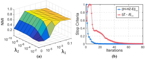
Parameter tuning. In our experiments, we set the dimensionality of latent representation as 200 and tune hyperparameters λ1 and λ2 from {10-5 , 10-4 , · · · , 10-1 , 100 } and {10-10 , 10-9 , · · · , 10-3 ,
10-2 }, respectively. Figure 1(a) shows the effect of changing values of λ1 and λ2 on clustering performance. We can observe that our method is less sensitive to λ2.
| Datasets | Metrics | Best View | 2nd Best | FeatConcate | CCA | KCCA | DCCA | FMR |
|---|---|---|---|---|---|---|---|---|
| Yale | NMI | 70.85±0.53 | 65.73±1.53 | 74.00±0.90 | 28.43±1.20 | 70.62±0.72 | 74.30±0.76 | 84.11±2.95 |
| ACC | 70.67±0.73 | 65.33±1.11 | 70.48±0.86 | 23.03±0.99 | 69.58±1.81 | 71.52±0.62 | 85.31±3.80 | |
| F-score | 55.06±1.15 | 46.81±1.50 | 56.76±1.48 | 8.67±0.65 | 50.17±1.29 | 57.12±1.03 | 72.17±4.57 | |
| RI | 94.37±0.18 | 93.05±0.19 | 94.37±0.22 | 87.72±0.17 | 93.83±0.88 | 94.59±0.16 | 95.23±0.64 | |
| MSRC-v1 | NMI | 56.15±0.67 | 51.73±0.28 | 42.88±1.00 | 9.60±0.91 | 39.97±0.44 | 66.04±0.09 | 71.68±1.51 |
| ACC | 67.81±0.65 | 60.84±0.00 | 48.35±2.18 | 24.68±0.68 | 56.37±0.23 | 76.09±0.08 | 82.08±1.44 | |
| F-score | 52.20±0.55 | 47.04±0.04 | 39.20±1.29 | 16.69±0.46 | 40.70±0.38 | 62.38±0.12 | 69.88±1.70 | |
| RI | 86.38±0.21 | 84.26±0.01 | 78.75±0.71 | 65.59±0.13 | 83.14±0.09 | 89.62±0.07 | 91.50±0.47 | |
| Notting | NMI | 71.92±0.00 | 66.64±0.00 | 79.80±0.13 | 14.50±0.00 | 60.27±0.00 | 65.46±0.00 | 80.91±3.85 |
| ACC | 86.36±0.00 | 78.55±0.00 | 87.05±0.01 | 30.36±0.00 | 72.00±0.00 | 80.73±0.00 | 89.47±4.43 | |
| F-score | 79.10±0.00 | 72.79±0.00 | 83.28±0.01 | 35.69±0.00 | 64.78±0.00 | 68.42±0.00 | 84.47±2.06 | |
| RI | 91.00±0.00 | 88.18±0.00 | 91.70±0.00 | 42.62±0.00 | 83.20±0.00 | 86.59±0.00 | 91.95±2.08 | |
| Reuters | NMI | 24.11±0.12 | 19.23±0.85 | 15.27±0.02 | 15.08±0.01 | 18.29±0.09 | 16.06±0.01 | 26.60±0.71 |
| ACC | 38.20±0.25 | 39.08±0.60 | 29.73±0.04 | 34.36±0.05 | 39.47±0.05 | 35.32±0.04 | 44.76±0.24 | |
| F-score | 32.24±0.32 | 31.63±0.10 | 28.56±0.00 | 26.69±0.02 | 29.19±0.04 | 27.55±0.03 | 37.03±0.52 | |
| RI | 71.27±0.04 | 70.93±0.03 | 59.42±0.03 | 66.93±0.03 | 71.69±0.02 | 68.77±0.03 | 71.66±0.36 | |
| BBCSport | NMI | 60.93±0.08 | 54.61±0.03 | 55.58±2.37 | 13.33±0.13 | 71.65±0.00 | 75.36±1.83 | 86.57±1.85 |
| ACC | 82.68±0.07 | 73.31±0.07 | 72.88±2.08 | 36.99±0.07 | 88.24±0.00 | 90.39±1.80 | 95.59±0.78 | |
| F-score | 70.77±0.08 | 59.75±0.08 | 66.73±1.75 | 38.60±0.00 | 79.72±0.00 | 81.18±1.16 | 91.60±1.36 | |
| RI | 86.42±0.04 | 85.82±0.02 | 83.93±1.06 | 30.50±0.00 | 90.76±0.00 | 91.55±0.22 | 96.03±0.64 | |
| Football | NMI | 85.22±0.00 | 81.42±0.44 | 83.47±0.55 | 53.21±0.40 | 82.42±0.79 | 87.92±0.65 | 89.96±0.75 |
| ACC | 84.27±0.00 | 75.97±2.45 | 79.60±0.87 | 45.56±1.28 | 81.53±0.90 | 81.45±0.63 | 88.02±1.43 | |
| F-score | 75.35±0.00 | 67.25±0.93 | 70.95±0.93 | 27.41±0.53 | 70.02±1.08 | 74.62±1.67 | 81.82±1.50 | |
| RI | 97.50±0.00 | 96.71±0.12 | 96.73±0.08 | 92.37±0.08 | 96.79±0.28 | 96.83±0.17 | 98.16±0.16 | |
| ANIMAL | NMI | 66.55±0.95 | 40.28±0.79 | 63.14±0.78 | 32.14±4.39 | 64.59±1.17 | 71.62±0.75 | 72.42±0.96 |
| ACC | 53.36±1.12 | 28.90±1.35 | 49.95±2.63 | 24.02±3.69 | 52.54±2.51 | 61.80±1.55 | 62.23±1.13 | |
| F-score | 48.05±1.35 | 18.23±0.99 | 43.30±2.16 | 8.71±1.31 | 40.83±1.98 | 52.93±2.14 | 54.96±1.31 | |
| RI | 97.25±0.16 | 95.36±0.06 | 96.75±0.16 | 71.32±2.60 | 96.25±0.19 | 97.52±0.15 | 97.58±0.63 |
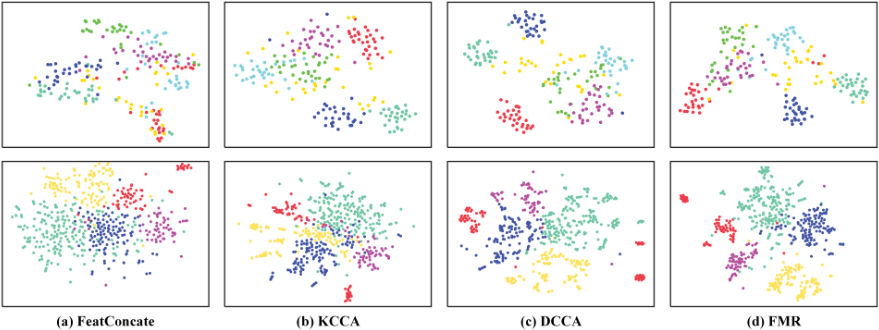
Figure 2: t-SNE visualizations of (a) FeatConcate, (b) KCCA, (c) DCCA, (d)FMR on MSRC-v1 (top row) and BBCSport (bottom row).
Convergence analysis. The convergence of inexact Augmented Lagrange Multiplier (ALM) method with three or more variable blocks is still difficult to theoretically prove [Liu et al., 2013], while there are six variable blocks in Algorithm 1. Fortunately, as shown in Figure 1(b), our method has strong convergence property in practice.
6 Conclusions
In this paper, we propose a novel method to flexibly learn a multi-view representation to improve subspace clustering. Different from data reconstruction within each single view, our method explores the complementary information among multiple views. Besides, we further extend the multi-view representation learning to nonlinear cases using HSIC. The learned latent representation can recover underlying cluster structure shared by multiple views and boost clustering performance greatly. Comprehensive evaluations on several benchmarks demonstrate the validity and superiority of our method.
Acknowledgements
This work was partly supported by National Natural Science Foundation of China (61602337, 61732011, 61702358), and Jiangsu Key Laboratory of Big Data Security & Intelligent Processing, NJUPT. Corresponding Author: Changqing Zhang.
@inproceedings{ijcai2019p404,
  title     = {Flexible Multi-View Representation Learning for Subspace Clustering},
  author    = {Li, Ruihuang and Zhang, Changqing and Hu, Qinghua and Zhu, Pengfei and Wang, Zheng},
  booktitle = {Proceedings of the Twenty-Eighth International Joint Conference on
               Artificial Intelligence, {IJCAI-19}},
  publisher = {International Joint Conferences on Artificial Intelligence Organization},
  editor    = {Sarit Kraus},
  pages     = {2916--2922},
  year      = {2019},
  month     = {8},
  note      = {Main track},
  doi       = {10.24963/ijcai.2019/404},
  url       = {https://doi.org/10.24963/ijcai.2019/404},
}
TY - CPAPER TI - Flexible Multi-View Representation Learning for Subspace Clustering AU - Li, Ruihuang AU - Zhang, Changqing AU - Hu, Qinghua AU - Zhu, Pengfei AU - Wang, Zheng T2 - Proceedings of the Twenty-Eighth International Joint Conference on Artificial Intelligence, IJCAI-19 PB - International Joint Conferences on Artificial Intelligence Organization PY - 2019 SP - 2916 EP - 2922 DO - 10.24963/ijcai.2019/404 UR - https://doi.org/10.24963/ijcai.2019/404 ER -Copied
Machine-readable versions of this paper, for tools and AI agents:





