Linear Time Complexity Time Series Clustering with Symbolic Pattern Forest

1 Introduction

Time series data widely exist in various scientific disciplines and industrial processes, thus the mining of time series data has attracted substantial interest. Time series clustering is one of the most important tasks in time series data mining. As an unsupervised technique, it does not require the data to be annotated or have class labels. Time series clustering has been applied in a variety of domains including astronomy [Rebbapragada et al., 2009], finance [Kumar et al., 2002], and so on [Aghabozorgi et al., 2015].

Time series clustering problem can be formulated as, given a set of unlabeled time series instances, to place them into homogeneous and separated groups. In this paper, we consider the partitional clustering problem of whole time series, i.e. we regard a time series instance as an object and cluster the time series objects into pairwise-disjoint groups.

With the advance of technologies, for example the sensors are becoming lighter, smaller and cheaper, hence widely embedded in various devices and machines, the amount of time series data becomes huge and the content is changing rapidly.

∗Contact Author

This requires the data mining algorithms to have low time complexity. Although there have been a wealth of work on time series clustering, little work is on providing a linear time solution with reasonable performance. Existing super-linear time complexity methods may not be applicable when the dataset is large, or when real-time analytics are required.

In this paper we propose a novel time series clustering algorithm, called Symbolic Pattern Forest (SPF), which has linear time complexity. The approach checks if some randomly selected symbolic patterns exist in the time series to partition the data instances. This partition process is executed multiple times, and the partitions are combined by ensemble to generate the final partition. We demonstrate that group structures in the data can emerge from the random partition process. Further analysis shows that the ensemble size needed to achieve good results does not directly depend on the input data size, and thus we can set the ensemble size to a proper fixed value for a specific data pattern.

The application of symbolic patterns in SPF has several benefits. Real-world time series often contain noise, amplitude change, phase-shift and irrelevant portion of data. The normalization step in symbolization can provide scaleinvariance against the amplitude change. In the average and symbolization step, some noise can be smoothed out. The symbolic patterns do not preserve the pattern location information in the time series, thus they are not affected by the phase-shift. If a time series contains a symbolic pattern in some portion, changing the values in other portion does not affect the appearance of the pattern, making SPF robust against irrelevant data.

Further, the utilization of symbolic patterns makes the pattern space finite, and we can use the symbolic patterns to partition the data without using a distance measure. Checking the boolean indicating array to assign clusters in SPF is efficient as boolean operations are very fast. Boolean values are space-efficient which can take more advantage of the CPU cache to speed up the program.

We evaluate the SPF algorithm on all 85 datasets in the well-known UCR time series archive [Chen et al., 2015], and compare with other state-of-the-art approaches with statistical analysis. The results show that SPF is better in accuracy compared with other rival methods.

The rest of the paper is organized as follows. Section 2 provides the background and related work. Section 3 provides the details of the proposed method and some analysis. The experimental evaluation is presented in Section 4, and Section 5 concludes the paper.

2 Background and RelatedWork

2.1 Definitions and Notations

This subsection provides the definitions and notations to precisely describe the problem under investigation and to present the proposed method.

Definition 2.1. A time series T is a ordered sequence of realvalue data points [t1, t2, . . . , tm], where m is the length of the time series.

Definition 2.2. A subsequence S of time series T is a sequence of contiguous values taken from T: S = [ti, ti+1, . . . , ti+l-1], where l is the length of the subsequence, 1 ≤ i ≤ m - l + 1 and 1 ≤ l ≤ m. All the subsequences of a certain length from a time series can be extracted using a sliding window of the same length from the first data point to the (m- l + 1)-th point.

Definition 2.3. Given a set of time series {Ti}ni=1 , where n is the number of time series instances, time series partitional clustering assigns a group relationship ci for each Ti, with ci = rj, j ∈ {1, 2, . . . , k}. rj is a group value and k is the number of clusters. Usually we have k ≪ m and k ≪ n. For presentation simplicity, we assume all the time series in the dataset have the same length m. The proposed algorithm in the paper can also work on datasets with varying-length time series.

2.2 RelatedWork

Some research on time series clustering is based on the kmeans algorithm [MacQueen, 1967]. In the k-means algorithm, the clustering group relationship is generated by an iterative refinement procedure. In initialization, k centroids are randomly selected. In each iteration, the distances from the instances to the centroids are computed and the instances are assigned to their nearest centroids. Centroids are then updated according to the new assignment.

In the standard k-means algorithm, Euclidean Distance (ED) [Faloutsos et al., 1994] is used as the distance metric and arithmetic mean is adopted to calculate the centroids. It is common for real-world time series data to contain phaseshift, warping, distortion and amplitude change. The simple ED may not be able to cope with these situations. Therefore, many time series distances measures are proposed [Wang et al., 2013], and one of the most popular ones is the Dynamic Time Warping (DTW) [Berndt and Clifford, 1994] which can align the data points from the two time series under comparison to find the optimal matching.

Methods of generating centroids under new time series distance measures have been proposed. Examples of these methods are NonLinear Alignment and Averaging Filters (NLAAF) [Gupta et al., 1996], Prioritized Shape Averaging (PSA) [Niennattrakul and Ratanamahatana, 2009] and Dynamic Time Warping Barycenter Averaging (DBA) [Petitjean et al., 2011].

K-shape [Paparrizos and Gravano, 2015] is one of the state-of-the-art time series algorithms based on k-means. It proposes a distance measure called Shape Based Distance (SBD), which is based on the cross-correlation of the time series. The centroids are generated by optimizing the within-cluster squared normalized cross-correlation between the centroids and the time series instances.

Another category of algorithms on time series clustering transform the time series into flat features and then apply classic clustering algorithms on the features to generate the cluster assignment. In [Kumar et al., 2005], the authors transform a time series into a bitmap, which is composed of the counts of all the symbolic patterns in time series. The bitmap representation provides a new distance measure for the classic clustering algorithms to run on time series data.

In the work by Zakaria et al. [Zakaria et al., 2012], the authors propose to enumerate all the subsequences in the time series dataset to select a subset of subsequences called Ushapelets that can best separate the data. The distances between the time series and these subsequences are computed and regarded as new feature values. Finally k-means is applied on the new feature values to get the clustering result. Although the shapelet-based method and the proposed technique both use local shapes in time series for clustering, they are quite different. The shapelet-based method adopts an iterative procedure to refine the clusters, while the proposed algorithm directly partitions the data and combines the partitions to get the clusters.

In a recent work [Zhang et al., 2016], instead of enumerating all the subsequences in the time series dataset, the shapelets are learned by optimizing an objective function.

2.3 Symbolic Aggregate Approximation

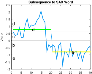
Since our method uses Symbolic Aggregate approXimation (SAX) [Lin et al., 2007] to transform a time series or subsequence to a symbolic pattern, we briefly introduce this technique. Figure 1 shows an example of transforming a subsequence to a symbolic pattern (SAX word). The subsequence is z-normalized and divided into ω segments (ω is 2 in this example). The mean value for each segment is computed (the green line and yellow line in the figure for the two segments respectively). These mean values are mapped to symbols according to a set of break points (the gray lines in the figure). These break points divide the value space in equal-probable regions. In this example the alphabet size of SAX is 4 (with an alphabet of 'a', 'b', 'c' and 'd'). The subsequence in the figure is transformed to the symbolic pattern "da". The alphabet size γ, number of segments (word length) ω, and subsequence length l are supplied by the users.

3 Symbolic Pattern Forest

For clarity, we present a small concrete example to illustrate the idea of the proposed method. Then we provide the formal description and analysis of the algorithm.

3.1 AConcrete Illustrative Example

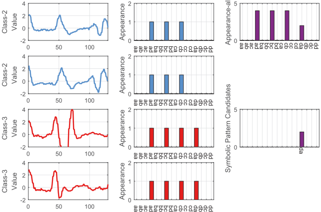
Figure 2 (Left) shows a small dataset of 4 time series instances belonging to 2 different classes (in blue and red respectively). These time series are taken from the FaceFour dataset from the UCR time series archive [Chen et al., 2015] and the time series in the dataset reflect the face outlines of different individuals under different conditions [Ratanamahatana and Keogh, 2004].

Given a set of SAX parameters, we can enumerate all possible symbolic patterns. The proposed method randomly picks a symbolic pattern from all available patterns, and checks if the pattern exists in the time series instances. More specifically, we use a sliding window of pre-defined length to go through the time series and extract all subsequences of the length. Each subsequence is transformed to a symbolic pattern and compared with the randomly chosen pattern.

This process is repeated multiple times so here we can optimize the process by scanning the time series in the beginning and storing the appearance of each pattern in a boolean indicating array. Boolean false (0) means the pattern does not appear in the time series, and boolean true (1) indicates the pattern appears. When checking a specific random pattern, we can directly look at the boolean array without needing to scan the time series again. Figure 2 (Center) shows the boolean indicating arrays for the four time series on the left respectively.

According to whether the time series contain a certain randomly selected pattern, the time series are partitioned into two groups. Those containing the pattern go to one group and the others are assigned to the other group. These two groups form two clusters. If the number of clusters k is more than 2, we perform the division with a new random symbolic pattern on the larger group. Previously chosen symbolic patterns are excluded from the pool of available pattern candidates. This process continues until we obtain k clusters, and the tree constructed from the procedure is called Symbolic Pattern Tree (SPT).

The above procedure are repeated multiple times, and multiple trees are constructed as a result, hence the name Symbolic Pattern Forest (SPF). Each tree is a partition of the data, and we combine the partitions in the forest by ensemble to get the final output partition.

The main idea of the symbolic pattern tree is that it uses a symbolic pattern to separate different time series groups. If a pattern appears in all the instances, it cannot separate the instances and thus we can exclude it from the symbolic pattern candidate pool. The same applies to the patterns that do not appear in any instances.

In SPF, the number of occurrences for each pattern in the dataset is counted, and the patterns with a count greater than an upper bound or less than a lower bound are excluded from the symbolic pattern candidate pool. The settings of these two bounds will be introduced later. Figure 2 (Right) shows the total occurrence count of each pattern in the dataset, as well as the final symbolic pattern candidate "da". SPF will select "da", which can separate the two classes into two clusters correctly.

3.2 SPF Algorithm

Cluster Ensemble

In SPF, each SPT generates a cluster assignment for all the time series instances, and these clusters are combined by ensemble to generate the final cluster assignment. Hybrid Bipartite Graph Formulation (HBGF) [Fern and Brodley, 2004] is adopted in SPF to perform the cluster ensemble. HBGF has a linear time complexity. The idea of HBGF is to build a graph model where the instances and clusters of the ensemble are the vertices. Partitioning the graph generates the ensemble consensus clusters. In our implementation, we use Metis [Karypis and Kumar, 1998] to partition the graph.

Efficient SAX Computation

In SPF, we need to compute the SAX symbolic pattern of each subsequence in the time series. The cumulative sum technique in [Li and Lin, 2017] is applied to calculate the symbolic pattern of an arbitrary subsequence in O(1) time (given the cumulative sums). The cumulative sum series U and cumulative squared sum series V of a time series T can be computed as: uj = ∑ji=1 ti, vj = ∑ji=1 t2i , where j = 1, . . . ,m and u0, v0 are set to 0.

For a subsequence x = [ti, . . . , ti+l-1], the mean value µx and standard deviation σx can be calculated as: µx = (ui+l - ui-1)/l, σx = √(vi+l - vi-1)/l - µ2x . x is divided in ω segments and each of the segment is mapped to a symbol. The normalized mean value of a segment y = [ti, . . . , tj] is µy = ((uj -ui-1)/(j-i+1)-µx)/σx. Then µy is mapped to a fixed break points region and transformed to a respective symbol [Lin et al., 2007].

Parameters of SAX

In SAX the number of segments ω, alphabet size γ, and subsequence length l are user-set parameters. In SPF, γ is set to 4 as previous research [Lin et al., 2007] suggests this value is suitable for most datasets. A grid search on the combinations of ω and l is performed. Each combination will generate a cluster assignment and all these assignments are combined by ensemble to give the final algorithm output. ω takes the values from wd = {3, 4, 5, 6, 7} and l takes the values from wl = {0.025, 0.05, 0.075, . . . , 1}m, i.e. an arithmetic sequence from 0.025m to m with a common difference of 0.025m, where m is the length of the time series. Duplicate values and values less than 10 are removed. In total at most 200 l and ω combinations are tested.

Algorithm 1 gives the pseudo-code of SPF. Given a time series dataset D, an ensemble size q and the number of clusters k, the algorithm returns a cluster assignment C as output.

Algorithm 1 Symbolic Pattern Forest (SPF)

Input: D: time series dataset q: ensemble size k: number of clusters Output: C: cluster assignment of D 1: T = loadData(D) 2: [U, V ] = CumulativeSum(T) 3: for each ω ∈ wd do 4: for each l ∈ wl do 5: SP = SymbolicPattern(T, ω, l, U, V ) 6: PC = PatternCount(SP) 7: SPC = F indCandidates(PC) 8: for i = 1 to q do 9: CA = SP T (SPC, SP, k) 10: ES.add(CA) 11: end for 12: CA2 = Ensemble(ES) 13: ES2.add(CA2) 14: end for 15: end for 16: C = Ensemble(ES2)

In Line 1, the dataset D is loaded and stored in T. Line 2 computes the cumulative sum U and cumulative squared sum V from T, which will be used to calculate the symbolic patterns. Line 3-4 perform the grid search on ω and l discussed before. Line 5 calculates the symbolic pattern appearance indicating boolean array SP. Line 6 counts the number of occurrence of each symbolic pattern and stores the result in PC. Line 7 takes the pattern count PC to select the symbolic pattern candidate SPC that will be used in the SPT random selection process. The patterns that have a count greater than an upper bound or less than a lower bound are removed from the candidate pool. In our method, we set the lower bound to 0.25 × n/k where n is the number of instances and k is the number of clusters. The upper bound is set to n-0.25 × n/k. These bounds are set so to remove non-distinguishing patterns according to our experiments.

In Line 8-11, SPT uses the symbolic pattern candidates to generate a cluster assignment CA, and CA is added to an ensemble set ES. This process is repeated q times. In Line 12, we combine the cluster assignments in ES by ensemble and get the consensus cluster assignment CA2. CA2 is added to the ensemble set ES2 in Line 13. Finally in Line 16, the cluster assignments in ES2 is combined by ensemble to receive the final cluster assignment C as the output of the algorithm.

3.3 Analysis of SPF

Time Complexity

Recall n denotes the number of time series instances, and m denotes the length of time series. k is considered as a constant much smaller than m and n. In Algorithm 1 the computation of cumulative sums takes O(nm) time. The number of grid search combinations is at most 200. It takes O(nm) time to obtain the symbolic pattern boolean indicating arrays and the symbolic pattern candidates. SPT takes O(n) time and the ensemble process also takes O(n) time. So the total time complexity of SPF is O(nm), which is linear to the input data size.

Effectiveness of SPF

In this subsection we show that if there exists a group structure in the dataset related to one pattern or some patterns, then SPF will output such group relationship. The intuition is that the unrelated patterns distribute uniformly among the instances so their effects cancel each other out in the ensemble, and only the structure on the related patterns is maintained and revealed. More formally, We have the following theorem:

Theorem 3.1. Consider two instances T1 and T2 in the same class, if they agree with each other on some related patterns, then SPF will put them in the same cluster.

Proof. Assume β is the percentage of related patterns in the symbolic candidate patterns. In the random selection process, if a related pattern is selected, then P(C(T1) = C(T2)) = 1, where P(·) is the probability function and C(·) is the cluster assignment function. If an unrelated pattern is selected, P(C(T1) = C(T2)) = P(C(T1) ̸= C(T2)) = 1/2. So overall P(C(T1) = C(T2)) = β × 1 + (1 - β) × 1/2 and P (C(T1) ̸= C(T2)) = (1 - β) × 1/2. We have:

Each tree is independent, according to the law of the large numbers, when we have sufficiently large ensemble size:

where Count(C(T1) = C(T2)) is the count of cases that T1 and T2 are in the same cluster. So in the ensemble result, T1 and T2 are assigned in the same cluster.

In the above analysis, we assume the ensemble size is sufficiently large, the following theorem quantifies how large the size should be.

Theorem3.2. Assume the ensemble size is q, the lower bound of q to receive a good clustering result is -2 lnα/β2 , where 1-α is the confidence level, β is the related pattern percentage in the symbolic pattern candidate pool.

Proof. Let X denote the random variable where there are X cases with C(T1) = C(T2). Then X follows the binomial distribution:

where p = P(C(T1) = C(T2)). Equation (2) should hold with high probability, so our goal can be formulated as:

where z = q/2, 1-α is the confidence level, e.g. 95%. Here considering Hoeffding's inequality [Hoeffding, 1994]:

where t ≥ 0. Considering E[ ¯X] = p, we have:

Let z = qp - qt, we have t = (qp - z)/q:

Recall z = q/2, p = β ×1+(1-β)×1/2, we can solve the above inequality and get:

Here is a concrete example of this boundary value: let the confidence level be 99% and assume 50% of the patterns in the pattern candidate pool are related patterns. So α = 0.01 and β = 0.5, we get q ≥ 36.84.

One observation from equation (9) is that the ensemble size lower bound does not directly depend on the number of instances n and time series length m. In the experiment part we will see the accuracy results do not change with fixed ensemble size and varying instances numbers and time series lengths, given the same data input type .

4 Experimental Evaluation

4.1 Experimental Setup

To evaluate the proposed algorithm, we run it on all 85 datasets from the UCR time series archive [Chen et al., 2015]. This public archive contains different types of labeled time series from various fields. Each dataset in the archive contains a training set and a testing set. We fuse both sets and use all the data in the experiment. The results of SPF are compared with other rival methods. The widely used k-means algorithm [MacQueen, 1967] is selected as the baseline. Standard kmeans adopts ED as the distance metric and uses arithmetic mean to calculate centroids. K-shape [Paparrizos and Gravano, 2015] introduced in Section 2 is selected for comparison as in [Paparrizos and Gravano, 2015] the authors show k-shape is superior to other state-of-the-art time series clustering algorithms (including those based on DTW).

The source code of k-shape and k-means are obtained from the author of [Paparrizos and Gravano, 2015] and the code is in Matlab. The number of iterations of k-shape and kmeans are set to 100 which is the same as in [Paparrizos and Gravano, 2015]. The ensemble size of SPF is set to 100 in all the experiments. k is set to equal the number of classes of the dataset in use. Following [Paparrizos and Gravano, 2015], we use the Rand Index to measure the accuracy of the clustering results. Rand Index is defined as: Rand Index = (TP + TN)/(TP + TN + FP + FN), where TP is the number of instances belonging to the same class and assigned in the same cluster, TN is the number of instances belonging to different classes and assigned in different clusters, FP is the number of instances belonging to different classes but assigned in the same cluster, and FN is the number of instances belonging to the same class but assigned in different clusters.

To verify the time complexity of SPF, we run it on the widely used CBF dataset [Saito and Coifman, 1994] of different sizes and record the average running time for each size. This dataset is a synthetic dataset, so with its underlying data generation rules in [Saito and Coifman, 1994], we can conveniently generate the datasets with different number of instances and time series lengths.

The C++ source code of SPF is available in the supplementary material 1 . The experiments are conducted in a batchprocessing cluster. A single core of AMD Opteron Processor 6276 (2299 MHz) and 16 GB memory are used.

1 http://mason.gmu.edu/∼xli22/SPF

4.2 Experimental Results

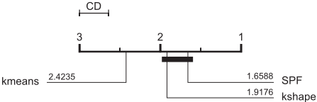
k-means, k-shape and SPF are run on the 85 datasets 10 times; the average running time and average Rand Index on each dataset are recorded. Due to space limitation, the results are not listed here and all the results are available in the supplementary material1 . Here we present the summarization of the comparison. Figure 3 shows the critical difference diagram [Demˇsar, 2006] (at 95% confidence level) for the Rand Index comparison. The value beside each method in the figure is the rank mean (lower is better) for the respective method. The methods that are connected by a bold bar have no significant difference.

From the figure one can see the accuracy of SPF is significantly better than that of k-means. SPF is also better than k-shape in rank mean, but the difference is not significant. So the overall accuracy of SPF is quite competitive. Performing the Wilcoxon signed rank test on the Rand Index result, the p-values between SPF and k-means, k-shape are 2.15 × 10-4 and 5.69 × 10-2 respectively. The conclusion from the Wilcoxon signed rank test coincides with that from the critical diagram.

The time complexities of k-means, k-shape and SPF are O(nm), O(max(nm2 ,m3 )), O(nm) respectively. Compared with k-means, SPF has the same time complexity but is significantly more accurate. Compared with k-shape, SPF has lower time complexity and slightly better accuracy. The total actual running time of k-means, k-shape and SPF on the 85 datasets are 1278, 19322, 1241 seconds respectively. Note that these methods are implemented in different languages so these time values just show how fast we can cluster the data using the available source code.

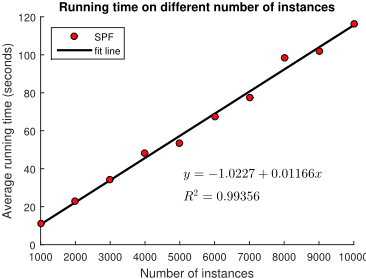
Figure 4 shows the average running time of SPF on the CBF datasets. The number of instances is changed from 1000 to 10000 and the length of time series is fixed at 1000. In the figure, the x-axis value is the number of instances and the y-axis value is the average running time of 30 runs. Linear regression curve fitting is performed on the data and the black line in the figure is the fit line. From the figure one can see the R2 value, which is the coefficient of determination of the fitting, is 0.99356. This value is very close to 1, indicating the average running time of SPF and the number of instances have a strong linear relationship.

Figure 5 gives the average running time of SPF on the CBF datasets of different lengths. The number of instances is fixed at 1000 and the length is changing from 1000 to 10000. Each time value in the figure is the average time of 30 runs. The coefficient of determination R2 value is 0.99923. This value is very close to 1, indicating the average running time of SPF

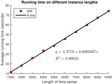
and the length of time series have a strong linear relationship. The above results coincide with the time complexity analysis in section 3.3. Also in the experiment we record the average Rand Index of SPF on different input combinations. The Rand Index values remain the same at 1 under all the cases. The ensemble size is fixed in the experiment, and this result is in accord with the analysis in section 3.3, that given a certain data type, the ensemble size to receive good accuracy results does not directly depend on the number of instances or time series lengths.

5 Conclusion

This paper presents a Symbolic Pattern Forest (SPF) algorithm for time series clustering. The method partitions the time series instances by checking some randomly selected symbolic patterns and the partitions of multiple runs are combined to give a final cluster assignment. Analysis is conducted on the time complexity and effectiveness of the algorithm. We evaluate the algorithm extensively on all 85 datasets from the UCR time series archive and the results show that SPF is very competitive compared with other rival methods.

Acknowledgments

The experiments were run on ARGO, a research computing cluster provided by the Office of Research Computing at George Mason University, VA. (URL: http://orc.gmu.edu)