
Worst-Case Discriminative Feature Selection
Proceedings of the Twenty-Eighth International Joint Conference on Artificial Intelligence. Main track. Pages 2973-2979.
https://doi.org/10.24963/ijcai.2019/412
Keywords
- Machine Learning: Feature Selection ; Learning Sparse Models
- Machine Learning: Classification
Abstract
Feature selection plays a critical role in data mining,
driven by increasing feature dimensionality in target problems. In this paper, we propose a new criterion for
discriminative feature selection, worst-case discriminative feature selection (WDFS).
Unlike Fisher Score and other methods based on the discriminative criteria
considering the overall (or average) separation
of data, WDFS adopts a new perspective called
worst-case view which arguably is more
suitable for classification applications. Specifically, WDFS directly maximizes the ratio of the
minimum of between-class variance of all class pairs over the maximum of within-class
variance, and thus it duly considers the separation of all classes. Otherwise, we
take a greedy strategy by finding one feature at a time, but it is very easy to
implement. Moreover, we also utilize the correlation between
features to help reduce the redundancy and extend WDFS to uncorrelated WDFS (UWDFS).
To evaluate the effectiveness of the proposed algorithm, we conduct
classification experiments on many real data sets. In the experiment, we respectively
use the original features and the score vectors of features over all class
pairs to calculate the correlation coefficients, and analyze the experimental
results in these two ways. Experimental results demonstrate the effectiveness
of WDFS and UWDFS.
- [Battiti, 1994] Roberto Battiti. Using mutual information for selecting features in supervised neural net learning. IEEE Transactions on Neural Networks, 5(4):537-550, 1994.
- [Ben-Bassat, 1982] Moshe Ben-Bassat. Pattern recognition and reduction of dimensionality. 1982.
- [Bian and Tao, 2011] Wei Bian and Dacheng Tao. Max-min distance analysis by using sequential sdp relaxation for di- mension reduction. IEEE Transactions on Pattern Analysis and Machine Intelligence, 33(5):1037-1050, 2011.
- [Cai et al., 2013] Xiao Cai, Feiping Nie, and Heng Huang. Exact top-k feature selection via ℓ 2,0 -norm constraint. In IJCAI, pages 1240-1246, 2013.
- [Dash and Liu, 1997] Manoranjan Dash and Huan Liu. Fea- ture selection for classification. Intelligent data analysis, 1(3):131-156, 1997.
- [Fisher, 1936] Ronald Aylmer Fisher. The use of multiple measuremens in taxonomic problems. Annals of Human Genetics, 7(2):179-188, 1936.
- [He et al., 2005] Xiaofei He, Deng Cai, and Partha Niyogi. Laplacian score for feature selection. In Advances in Neu- ral Information Processing Systems, pages 507-514, 2005.
- [Kohavi and John, 1997] Ron Kohavi and George H. John. Wrappers for feature subset selection. Artificial Intelli- gence, 97(1):273-324, 1997.
- [Loog et al., 2001] Marco Loog, Robert P. W. Duin, and Reinhold Haeb-Umbach. Multiclass linear dimension re- duction by weighted pairwise fisher criteria. IEEE Trans- actions on Pattern Analysis and Machine Intelligence, 23(7):762-766, 2001.
- [Masaeli et al., 2010] Mahdokht Masaeli, Jennifer G. Dy, and Glenn M. Fung. From transformation-based dimen- sionality reduction to feature selection. In ICML, pages 751-758, 2010.
- [Nie et al., 2008] Feiping Nie, Shiming Xiang, Yangqing Jia, Changshui Zhang, and Shuicheng Yan. Trace ratio crite- rion for feature selection. In AAAI, volume 2, pages 671- 676, 2008.
- [Nie et al., 2010] Feiping Nie, Heng Huang, Xiao Cai, and Chris Ding. Efficient and robust feature selection via join- t ℓ 2,1 -norms minimization. In International Conference on Neural Information Processing Systems, pages 1813- 1821, 2010.
- [Pena and Nilsson, 2010] Jose M. Pena and Roland Nilsson. On the complexity of discrete feature selection for optimal classification. IEEE Transactions on Pattern Analysis and Machine Intelligence, 32(8):1517-1522, 2010.
- [Peng et al., 2005] Hanchuan Peng, Fuhui Long, and Chris H. Q. Ding. Feature selection based on mutual informa- tion criteria of max-dependency, max-relevance, and min- redundancy. IEEE Transactions on Pattern Analysis and Machine Intelligence, 27(8):1226-1238, 2005.
- [Raileanu and Stoffel, 2004] Laura Elena Raileanu and Kil- ian Stoffel. Theoretical comparison between the gini index and information gain criteria. Annals of Mathematics and Artificial Intelligence, 41(1):77-93, 2004.
- [Rao, 1948] C. Radhakrishna Rao. The utilization of mul- tiple measurements in problems of biological classifica- tion. Journal of the royal statistical society series b- methodological, 10(2):159-193, 1948.
- [Robnik et al., 2003] Robnik, Marko Ikonja, and Igor Kononenko. Theoretical and empirical analysis of relieff and rrelieff. Machine Learning, 53(1-2):23-69, 2003.
- [Romero and Sopena, 2008] Enrique Romero and Josep Maria Sopena. Performing feature selection with multilayer perceptrons. IEEE Transactions on Neural Networks, 19(3):431-441, 2008.
- [Su et al., 2018] Bing Su, Xiaoqing Ding, Changsong Liu, and Ying Wu. Heteroscedastic max-min distance analy- sis for dimensionality reduction. IEEE Transactions on Image Processing, 27(8):4052-4065, 2018.
- [Tao et al., 2016] Hong Tao, Chenping Hou, Feiping Nie, Yuanyuan Jiao, and Dongyun Yi. Effective discriminative feature selection with nontrivial solution. IEEE Transac- tions on Neural Networks, 27(4):796-808, 2016.
- [Wang et al., 2008] Lipo Wang, Nina Zhou, and Feng Chu. A general wrapper approach to selection of class- dependent features. IEEE Transactions on Neural Net- works, 19(7):1267-1278, 2008.
- [Yu and Liu, 2004] Lei Yu and Huan Liu. Efficient feature s- election via analysis of relevance and redundancy. Journal of Machine Learning Research, 5:1205-1224, 2004.
- [Yu and Yeung, 2010] Zhang Yu and Dit Yan Yeung. Worst- case linear discriminant analysis. In International Confer- ence on Neural Information Processing Systems, 2010.
- [Zhang et al., 2018] Rui Zhang, Feiping Nie, and Xuelong Li. Self-weighted supervised discriminative feature selec- tion. IEEE Transactions on Neural Networks, 29:3913- 3918, 2018.
References were extracted automatically from the PDF and may contain errors.
Full text extracted automatically from the PDF; figures, tables and equations may differ. The PDF is the version of record.
1 Introduction
Nowadays, the dimensionality of the data involved many realworld applications has increased explosively. The presence of many irrelevant and redundant features [Ben-Bassat, 1982] tends to make a learning model overfitting, resulting in its performance degenerates. Dimensionality reduction is one of the most popular techniques to help address this problem. Feature selection is a widely employed technique for reducing dimensionality among practitioners. It aims to select a small number of significant and useful original features without any transformation. Thus, feature selection could maintain the original representation of variables, which leads to better readability and interpretability. Many efforts have been devoted to the research in feature selection during the past few years [Romero and Sopena, 2008] [Pena and Nilsson, 2010].
∗Contact Author: Q. Gao. (qxgao@xidian.edu.cn)
†Contact Author: F. Nie. (feipingnie@gmail.com)
According to how the learning algorithm is integrated into the process of evaluating and selecting features, feature selection methods can be roughly categorized as wrapper methods [Kohavi and John, 1997] [Wang et al., 2008], embedded methods [Nie et al., 2010] [Cai et al., 2013] and filter methods. The wrapper methods and embedded methods are tightly coupled with the specific classifier, they always have better performance than filter methods on the particular classifier but not on the other classifiers. Different from wrapper and embedded methods, the filter-type methods, which evaluate features based on a certain criterion, are absolutely independent on any classifier. Most existing filter-type feature selection methods conducted the selection process in the manner of feature ranking [Robnik et al., 2003] [Raileanu and Stoffel, 2004] or feature subset evaluation [Nie et al., 2008]. Methods based on the feature ranking compute the relevance of a feature with respect to the class label distribution of data. In this paper, we propose a new filter-type feature selection method in the manner of feature ranking.
For the classification problem, feature selection aims to select subset of highly discriminant features. In other words, it selects features that are capable of discriminating samples that belong to different classes. Fisher discriminant criterion [Fisher, 1936] is probably the most widely used one. One of the most representative algorithms is Fisher score [He et al., 2005], which optimizes the so-called Fisher criterion that maximizes the ratio of between-class scatter over within-class scatter in a individual feature level. On this basis, the Laplacian score [He et al., 2005] also consider the feature ability of preserving the local manifold structure. Then Trace Ratio [Nie et al., 2008] was proposed to improve the computational efficiency of Fisher score, which selects a feature subset based on the corresponding subset-level score that is calculated in a Trace Ratio form. Moreover, there are many feature selection method, combining the popular transformationbased dimensionality reduction method linear discriminant analysis (LDA) and sparsity regularization [Masaeli et al., 2010]. For example, Discriminative Feature Selection (DF- S) [Tao et al., 2016] imposes the row sparsity on the transformation matrix of LDA through ℓ2,1-norm regularization to achieve feature selection. Zhang et al. proposed a selfweighted supervised discriminative feature selection (SSDFS) method [Zhang et al., 2018], which constrains the transformation matrix to be orthogonal and introduces the ℓ2,1norm regularization to select features.
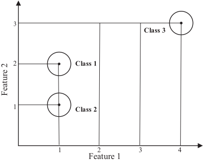
However, according to the definition of between-class scatter, the aforementioned methods actually maximize the average of all pairwise distances between classes [Bian and Tao, 2011] [Su et al., 2018]. This may cause the so-called class separation problem [Loog et al., 2001]. Specifically, these methods tend to pay close attention to classes with larger distances, but ignore those with smaller distances, resulting in the overlap of neighboring classes in the lower-dimensional space. An example to illustrate the class separation problem is shown in Figure 1, where class 1 and class 2 locate closely to each other while class 3 is far away from them, and all classes have the same covariance. We can directly see that the Feature 2 could easily separates three class, while the Feature 1 would result in a complete confusion of class 1 and class 2. But according to the muti-class Fisher certeria [Rao, 1948], the average of pairwise distances between classes is maximized in the Feature 1.
Due to the fact that many feature selection methods based on the discriminative criteria usually consider the overall (or average) separation of data, thus they cannot guarantee the separation (as best as possible) of any class pairs. Thus, we propose a new criterion for discriminative feature selection, namely worst-case discriminative feature selection (WDFS), which adopt a worst-case view [Yu and Yeung, 2010] but the average view. Specifically, WDFS directly maximizes the ratio of the minimum of between-class variance of all class pairs over the maximum of within-class variance, and thus it duly considers the separation of all classes. For the solution, we take a greedy strategy by finding one feature at a time, but that is very easy to implement. Moreover, in order to reduce the redundancy of selected feature subset, we extend WDFS to uncorrelated WDFS (UWDFS) with the help of the correlation between features. Finally, in the experiment, we respectively use the original features and the score vectors of features over all class pairs to calculate the correlation coefficients, and analyze the experimental results in these two ways. Our contribution are summarized as follows:
- Our method WDFS duly considers the separation of all classes, which adopts a new view called worst-case view different from the conventional average view.
- Considering the feature evaluation mechanism of the WDFS model, we propose a method to help reduce the redundancy, which only needs to calculate the correlation coefficients between features or feature score vectors.
- Although we take a greedy strategy by finding one feature at a time, that is very easy to implement with low computational complexity.
2 RelatedWorks
2.1 Fisher Score
Given a set of N data points {xk ∈ Rd×1 |k = 1, · · · ,N } which are sampled from C classes. The within-class matrix Sw and between-class matrix Sb are defined as
where ni denotes the number of samples in the i - th class, µi denotes the mean of the i - th class, and xip denotes the p - th sample in the i - th class.
To specify the selected features in the procedure of feature selection, we equip the conventional transportation matrix with an explainable structure to specify the selected features, namely selective matrix. Next, we will go into details. First, concatenate the dataset {x1, x2, . . . , xN} to a matrix X=[x1, x2, . . . , xN] ∈ Rd×N . Then let fr T ∈ R1×N denotes the r-th row of X, i.e. the r-th feature of the dataset, and then let F = XT = [f1, f2 . . . , fd] ∈ RN×d . Formally, for a feature subset FI ∈ F, we could define the corresponding selective matrix as
where wI(k) ∈ Rd×1 (k = 1, 2, . . . ,m ≤ d) refers to a column vector whose components are all 0 expect 1 for the I (k) - th one. Note that this WI is indeed a column-fullrank transformation matrix. With the selective matrix WI, the process of feature selection could be expressed as
Then the model of Fisher Score could be formulated as
It should be noted that each feature is evaluated individually. It is easy to see that the model in the Eq. (5) consider the overall (or average) separation of data, thus it cannot guarantee the separation (as best as possible) of any class pairs.
2.2 Redundancy
The Redundancy (feature-feature) analysis has been another concerned part of supervised filter models, which has many similarities to the Relevance (feature-class) in term of measurement. Yu and Liu [Yu and Liu, 2004] explored further feature redundancy, and more restrictively defined relevant features as any feature that is neither irrelevant nor redundant to the target concept. The independence or complementarity of one feature can be defined based on correlation coefficient, mutual information, or any criterion characterizing feature redundancy. Many models use Euclidean distance, Pearson correlation [Battiti, 1994], and information measures for redundancy analysis. Some feature selection methods seek to remove redundant features while others do not. A classical criterion for feature selection based on relevance and redundancy analysis is Max-Relevance and Min-Redundancy (mRMR) [Bian and Tao, 2011], which maximizes the correlation between features and categorical variables while minimizing the correlation between features by measuring the mutual information.
3 Approach
In order to guarantee the separation (as best as possible) of any class pairs, we propose a new criterion for discriminative feature selection, worst-case discriminative feature selection (WDFS) in the subsection 3.1. Unlike Fisher Score and other methods based on the discriminative criteria considering the overall (or average) separation of data, WDFS adopts a worst-case view which duly considers the separation of all classes. Specifically, WDFS directly maximizes the ratio of the minimum of between-class variance of all class pairs over the maximum of within-class variance of all classes.
Apart from the analysis of relevance (feature-class), the analysis of redundancy (feature-feature) is another crucial part of supervised filter models. This work simply uses the correlation coefficient to help reduce redundancy among features. Then WDFS is extended to uncorrelated WDFS (UWDFS) in the subsection 3.2.
3.1 Worst-Case Discriminative Feature Selection
In the Eq. (1), due to the fact that µ = 1N c∑ i=1 niµi, thus the equation (1) would be equal to the following equation by simple derivation.
Next, we define the between-class matrix Si,j b for the class pair (i, j) and the within-class matrix Siw as
where µi denotes the mean of the i - th class, and denotes the sample in the class. Similarly, based on the Fisher discriminative criterion, we formulate the model of worst-case
Algorithm 1 WDFS
Input: Train dataset {(xi, yi) |i = 1, 2, . . . ,N }, wherein xi ∈ Rd×1 and yi ∈ {1, 2, · · · , C}, the selected number m. Initialize: Concatenate the dataset {x1, x2, . . . , xN} to a matrix X=[x1, x2, . . . , xN] ∈ Rd×N , and let F = XT = [f1, f2 . . . , fd].
Output: Selective matrix WI ∈ Rd×m.
- 1: Calculate the within-class matrix Siw for all class by the Eq. (7), and between-class matrix Si,j b for all class pair (i, j) , 1 ≤ i < j ≤ C by the Eq. (8).
- 2: For each feature, calculate the score score(fr),r = 1, 2, . . . , d by the Eq. (10).
- 3: Sort the scores of all features.
- 4: Select the m feature indexes corresponding to the first m largest feature scores and construct the corresponding selective matrix WI .
discriminative feature selection as
It should be noted that each feature is evaluated individually. Thus, we could a greedy strategy by finding one feature at a time to solve this optimization problem. Define the score of the r - th feature in F as
where wr is a selective vector corresponding to the r - th feature in F. For clarity, Algorithm 1 lists the pseudo code of solving the model WDFS.
3.2 UncorrelatedWDFS
In this subsection, we extend WDFS to Uncorrelated WDFS (UWDFS) by calculating correlation coefficients between features to help reduce the redundancy. For a feature pair (fi, fj), we define the correlation coefficient as
where σ (·) is a scalar function, which calculate the similarity (correlation) between two vectors. It is worth noting that the larger correlation coefficient means a greater redundancy between features.
Moreover, according to the aforementioned analysis, we have that WDFS evaluates feature individually. Then we calculate the correlation coefficient between each feature of the rest features (current candidate feature subset except for the feature with the largest score) and the feature with the largest score. These correlation coefficients can further be used to calculate the weights, indicating the importance difference among the rest features.
Specifically, suppose the current selected feature subset be Fk = {fI(1), fI(2), · · · , fI(k)} ⊂ F, and its complement, namely the candidate feature set, could be defined as
Algorithm 2 UWDFS
Input: Train dataset {(xi, yi) |i = 1, 2, . . . ,N }, wherein xi ∈ Rd×1 and yi ∈ {1, 2, · · · , C}, the selected number m. Initialize: Concatenate the dataset {x1, x2, . . . , xN} to a matrix X=[x1, x2, . . . , xN] ∈ Rd×N , and let F = XT = [f1, f2 . . . , fd].
Output: Selective matrix WI ∈ Rd×m.
- 1: Calculate the score vector s(0) by the Eq. (10).
- 2: for k = 1 to mdo
- 3: Find the feature fI(k) = fmax and remove it from the current candidate feature subset F c k , then obtain the new candidate feature subset F c k+1 .
- 4: Calculate the correlation coefficient vector
- 5: ρ = [ρ1, ρ2, · · · , ρd-k-1] between F c k+1 and current fmax by the Eq. (11).
- 6: Update the score vector by the Eq. (16), then s(k) = [s(k) 1 , s(k) 2 , · · · , s(k) d-k-1 ]
7: end for
- 8: Construct the selective matrixWI corresponding to the selected feature subset {fI(1), fI(2), · · · , fI(m)}.
Here, we take the process of selecting the first two features as an example. The main steps are summarized as follows.
Step 1 : When k = 0, i.e. F0 = ∅, we calculate the score for ˜ fr (r = 1, · · · , d) by the Eq. (10), then we get a score vector
where sr (r = 1, · · · , d) is a scalar. Then we find the feature fmax with the largest score as
Then we obtain F c 1 = F - {fI(1)} = { ˜ f1, ˜ f2, · · · , ˜ fd-1}. Step 2 : We calculate the correlation coefficient between ˜ fr (r = 1, · · · , d-1) and fmax = fI(1) by the Eq. (11). Then we get the correlation coefficient vector
Then we can use the 1 - ρr (r = 1, · · · , d - 1) as the weight of ˜ fr. This is consistent with the assumption that a less redundant feature should be assigned a larger weight, while a more redundant feature should be assigned a smaller weight. Finally, we update the score of ˜ fr (r = 1, · · · , d-1) as
Then the new score vector is s(1) = [s(1) 1 , s(1) 2 , · · · , s(1) d-1 ] and the new fmax is
So far, we have described a complete operation of selecting a feature in UWDFS. For clarity, Algorithm 2 lists the pseudo code of solving the model UWDFS.
| Dataset | Instances | Features | Classes | Type |
|---|---|---|---|---|
| COIL20 | 1440 | 1024 | 20 | Object Image |
| USPS | 7000 | 256 | 10 | HandWritten Image |
| ORL | 400 | 1024 | 40 | Face Image |
| UMIST | 575 | 1024 | 20 | Face Image |
| LUNG | 203 | 3312 | 5 | Biological |
4 Experiments
In this section, we will validate our proposed methods compared with other state-of-the-art methods on five datasets.
4.1 Datasets Descriptions
These datasets include one object image dataset, COIL20, USPS, two face image datasets ORL 1 and UMIST, and one biological gene expression microarray dataset, lung cancer (LUNG). (The COIL20, USPS and LUNG datasets are download from the Internet 2 ). We summarize the statistics of the data sets in Table 2 and briefly introduce them as follows.
- COIL20 contains 1440 images of 20 objects. The images of each object were taken 5 degrees apart as the object is rotated on a turntable, and each object has 72 images.
- The original USPS handwritten digit database contains 9298 images. In this paper, we select a balanced random sample of the original data set.
- ORL consists of 400 face images. There are ten different images of each of 40 distinct subjects. For some subjects, the images were taken at different times with varying lighting, different facial expressions, and facial details.
- UMIST contains 20 persons and totally 575 images. The number of data in each class is between 10 and 24.
- LUNG is composed of 203 samples in five classes with 139, 21, 20, 6, and 17 samples, respectively. Each sample has 12600 genes. The genes with standard deviations smaller than 50 expression units were removed and the remaining data set contains 203 samples with 3312 genes.
4.2 Reducing Feature Redundancy
A redundant feature does not add anything new to the target concept [Dash and Liu, 1997]. Thus, removing redundancy is straightforward when we require the number of selected features is as small as possible. Actually, we want the preserved features to be informative and complemental to each other. Considering that our proposed method selects one feature at a time, so we simply uses the correlation criteria to help reduce redundancy among features. The Pearson correlation coefficient [Battiti, 1994] is one of the simplest criteria. Moreover, in the experiment, we also try to use the score vectors over all class pairs instead of original feature as the input for calculating the correlation coefficients. The corresponding calculation formulas are as follows.
1 http://www.zjucadcg.cn/dengcai/Data/FaceData.html
2 http://featureselection.asu.edu/datasets.php
| Dataset | Average accuracy(%) of top 20 features | Average accuracy(%) of top 40 features | ||||||||
|---|---|---|---|---|---|---|---|---|---|---|
| Methods | COIL20 | USPS | ORL | UMIST | LUNG | COIL20 | USPS | ORL | UMIST | LUNG |
| RALMFS | 91.33 | 80.93 | 65.60 | 91.16 | 83.90 | 96.42 | 87.47 | 79.95 | 93.54 | 85.30 |
| ±3.97 | ±4.02 | ±6.04 | ±2.57 | ±5.47 | ±0.88 | ±2.65 | ±2.58 | ±1.84 | ±2.83 | |
| mRMR | 94.26 | 38.94 | 66.85 | 87.23 | 84.70 | 96.56 | 47.19 | 73.00 | 92.11 | 89.70 |
| ±1.67 | ±2.12 | ±4.31 | ±3.62 | ±2.06 | ±0.95 | ±1.78 | ±2.47 | ±1.89 | ±3.02 | |
| RFS | 88.25 | 82.95 | 68.55 | 90.07 | 87.30 | 95.61 | 90.45 | 76.70 | 93.54 | 90.50 |
| ±5.17 | ±3.06 | ±2.01 | ±2.99 | ±4.64 | ±2.70 | ±1.92 | ±3.28 | ±1.60 | ±2.32 | |
| TR | 58.83 | 73.38 | 60.05 | 83.79 | 81.50 | 90.28 | 85.44 | 76.50 | 92.49 | 86.70 |
| ±15.37 | ±1.00 | ±3.26 | ±4.88 | ±4.20 | ±1.95 | ±0.83 | ±3.73 | ±2.21 | ±2.41 | |
| DFS | 95.57 | 81.19 | 67.40 | 90.81 | 86.30 | 97.68 | 91.07 | 77.05 | 94.18 | 90.70 |
| ±1.47 | ±5.00 | ±3.65 | ±3.62 | ±5.36 | ±0.62 | ±1.88 | ±3.17 | ±1.81 | ±4.65 | |
| FisherScore | 58.83 | 73.38 | 60.05 | 83.79 | 81.50 | 90.28 | 85.44 | 76.50 | 92.49 | 86.70 |
| ±15.37 | ±1.00 | ±3.26 | ±4.88 | ±4.20 | ±1.95 | ±0.83 | ±3.73 | ±2.21 | ±2.41 | |
| Ours-WDFS | 96.13 | 87.75 | 73.65 | 90.63 | 89.40 | 97.90 | 93.40 | 83.25 | 94.18 | 90.90 |
| ±1.50 | ±1.63 | ±2.37 | ±3.38 | ±3.95 | ±1.02 | ±0.90 | ±3.44 | ±2.01 | ±2.60 | |
| Ours-UWDFS-1 | 96.96 | 91.09 | 70.70 | 92.39 | 84.40 | 98.68 | 94.52 | 79.90 | 94.77 | 84.00 |
| ±0.54 | ±1.19 | ±4.87 | ±1.53 | ±3.17 | ±0.44 | ±0.53 | ±3.59 | ±1.80 | ±3.33 | |
| Ours-UWDFS-2 | 97.25 | 90.47 | 73.80 | 92.70 | 89.30 | 98.68 | 94.24 | 82.65 | 95.61 | 91.20 |
| ±0.94 | ±1.24 | ±4.84 | ±1.55 | ±2.67 | ±0.54 | ±0.43 | ±3.49 | ±1.66 | ±2.35 | |
- Pearson correlation coefficient
where a and b are two vectors.
(2) The score vector over all class pairs
For the feature fr, similar to its score in the Eq. (10), we could define the corresponding score vector vr ∈ R C(C-1) 2 over all class pairs as
| Dataset | Average accuracy(%) of top 60 features | Average accuracy(%) of top 80 features | ||||||||
|---|---|---|---|---|---|---|---|---|---|---|
| Methods | COIL20 | USPS | ORL | UMIST | LUNG | COIL20 | USPS | ORL | UMIST | LUNG |
| RALMFS | 96.97 | 90.57 | 80.45 | 95.44 | 88.60 | 97.75 | 92.58 | 83.75 | 95.96 | 89.10 |
| ±0.92 | ±1.98 | ±3.30 | ±0.95 | ±3.20 | ±0.64 | ±1.34 | ±3.16 | ±1.22 | ±3.14 | |
| mRMR | 97.10 | 57.63 | 77.85 | 93.86 | 90.20 | 97.61 | 66.35 | 80.20 | 94.95 | 90.90 |
| ±0.76 | ±1.88 | ±2.15 | ±1.74 | ±1.75 | ±0.57 | ±1.04 | ±3.55 | ±1.54 | ±1.85 | |
| RFS | 97.07 | 92.40 | 79.05 | 94.32 | 91.20 | 97.86 | 93.45 | 80.30 | 94.42 | 91.60 |
| ±1.10 | ±1.31 | ±3.28 | ±1.76 | ±1.69 | ±0.81 | ±1.02 | ±3.34 | ±1.78 | ±2.12 | |
| TR | 94.33 | 89.22 | 82.20 | 94.98 | 88.60 | 95.58 | 92.45 | 86.60 | 96.14 | 90.70 |
| ±0.88 | ±0.79 | ±2.66 | ±2.40 | ±3.17 | ±0.63 | ±0.80 | ±1.43 | ±1.96 | ±2.50 | |
| DFS | 98.36 | 93.69 | 81.70 | 94.81 | 90.90 | 98.50 | 94.95 | 83.35 | 95.72 | 91.60 |
| ±0.72 | ±0.87 | ±2.55 | ±1.89 | ±3.33 | ±0.81 | ±0.52 | ±2.31 | ±1.77 | ±3.50 | |
| FisherScore | 94.33 | 89.22 | 82.20 | 94.98 | 88.60 | 95.58 | 92.45 | 86.60 | 96.14 | 90.70 |
| ±0.88 | ±0.79 | ±2.66 | ±2.40 | ±3.17 | ±0.63 | ±0.80 | ±1.43 | ±1.96 | ±2.50 | |
| Ours-WDFS | 98.54 | 94.76 | 86.20 | 95.44 | 91.50 | 98.76 | 95.26 | 86.95 | 95.58 | 92.20 |
| ±0.90 | ±0.84 | ±2.36 | ±1.34 | ±3.27 | ±0.81 | ±0.60 | ±3.62 | ±1.27 | ±2.04 | |
| Ours-UWDFS-1 | 98.75 | 95.28 | 82.75 | 95.51 | 83.00 | 98.99 | 95.55 | 84.00 | 95.93 | 82.60 |
| ±0.57 | ±0.36 | ±3.16 | ±1.26 | ±2.31 | ±0.40 | ±0.43 | ±3.90 | ±1.26 | ±2.72 | |
| Ours-UWDFS-2 | 98.92 | 95.11 | 84.50 | 96.07 | 92.30 | 99.13 | 95.42 | 84.30 | 96.32 | 92.80 |
| ±0.28 | ±0.32 | ±3.70 | ±1.70 | ±2.63 | ±0.36 | ±0.22 | ±3.50 | ±1.35 | ±2.20 | |
4.3 Comparison Algorithms and Parameter Setting
In our experiments, we compare our methods (WDFS and UWDFS) with other five methods, including RALMFS [Cai et al., 2013], mRMR [Peng et al., 2005], RFS [Nie et al., 2010], DFS [Tao et al., 2016], TR[Nie et al., 2008] and FisherScore [He et al., 2005]. (The code of mRMR, TR and FisherScore are downloaded from the ASU feature selection repository 3 and the code of DFS is implemented by ourselves in Python2.7.) Among them, RALMFS and RFS algorithms are embedded methods based on the linear regression model. The other methods belong to filter-type methods and except mRMR are all based on the Fisher discriminant criterion. Moreover, we respectively use the original features and the score vectors of features over all class pairs to calculate the correlation coefficients for UWDFS. For clarity, we call them UWDFS-1 and UWDFS-1 respectively.
We randomly divide each dataset into two parts that are approximately equal, one for training and the other for testing, and we repeat each group experiment for ten times. For the sake of simplicity and justice, we use the 1NN calssifier for classification and Euclidean distance as the metric and let the number of selected features be between 10 and 100 with an interval of 10.(There is no ideal method for choosing the dimension of the feature space.) In particular, the trade-off parameters in DFS and RFS, the trade-off parameters in DFS and RFS are set α from [1e - 6, 1e - 4, 1e - 3, 1e - 2, 0.1, 1, 10, 100, 1e3, 1e4].
4.4 Results Analysis
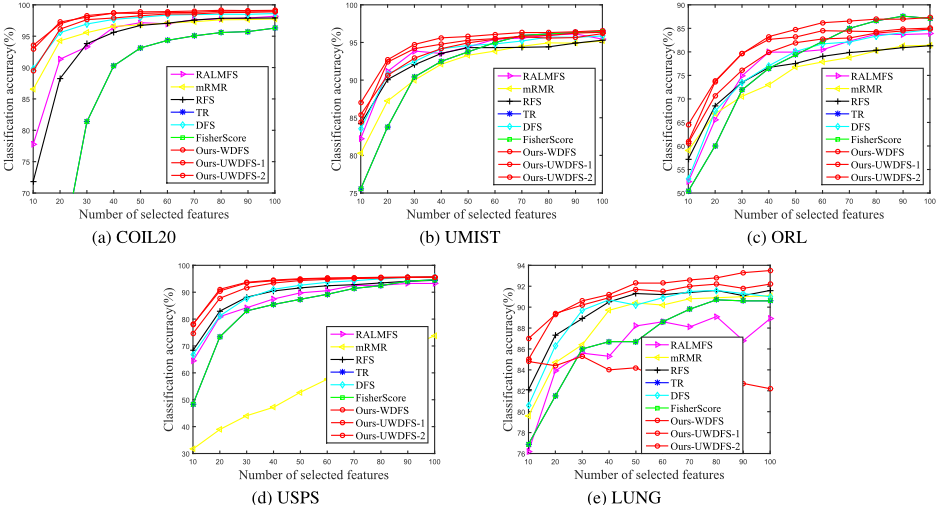
Figure 2 shows the average classification accuracy vs. the number of selected features on six datasets with five different methods. Tables 1 and 3 list the average classification accuracy and the corresponding standard deviation, using the top 20, 40, 60 and 80 features respectively. As can be seen in the experimental results, we have that
3 http://featureselection.asu.edu/index.php
- As shown in Figure 2, with the increase in the number of selected features, the trends of average classification accuracy of different methods almost have a steady rise on different datasets. With the specific values in Tables1 and 3, we can see that our methods have a better classification performance with minor exceptions. Particularly, our methods trumps all the other algorithms at the small number of features with a noticeable rise.
- On the ORL dataset, WDFS has better classification results than the other methods in most feature numbers. Our Uncorrelated WDFS is almost inferior to the WDFS algorithm. This may be an indication that the decorrelation process is working in a bad way, resulting in removing some weakly relevant and redundant features.
- Comparing the model UWDFS-1 with UWDFS-2, we can see that UWDFS-2 always has better performance than UWDFS-1. Especially on the LUNG dataset, UWDFS-2 shows a steady rise but UWDFS-1 has a completely opposite trend.
5 Conclusions
In this paper, we propose a new criterion for discriminative feature selection, worst-case discriminative feature selection (WDFS). Based on a worst-case view, WDFS duly considers the separation of all classes by maximizing the ratio of the minimum of between-class variance of all class pairs over the maximum of within-class variance. Moreover, we also utilize the correlation between features to help reduce the redundancy and extend WDFS to uncorrelated WDFS (UWDFS). Last but not least, the solution process in our model is simple and effective. Experimental results demonstrate the effectiveness of WDFS and UWDFS.
Acknowledgements
This work is supported by National Natural Science Foundation of China under Grant 61773302, Innovation Fund of Xidian University No.10221150004, China Postdoctoral Science Foundation (Grant 2019M653564) and the Fundamental Research Funds for the Central Universities.
@inproceedings{ijcai2019p412,
  title     = {Worst-Case Discriminative Feature Selection},
  author    = {Liao, Shuangli and Gao, Quanxue and Nie, Feiping and Liu, Yang and Zhang, Xiangdong},
  booktitle = {Proceedings of the Twenty-Eighth International Joint Conference on
               Artificial Intelligence, {IJCAI-19}},
  publisher = {International Joint Conferences on Artificial Intelligence Organization},
  editor    = {Sarit Kraus},
  pages     = {2973--2979},
  year      = {2019},
  month     = {8},
  note      = {Main track},
  doi       = {10.24963/ijcai.2019/412},
  url       = {https://doi.org/10.24963/ijcai.2019/412},
}
TY - CPAPER TI - Worst-Case Discriminative Feature Selection AU - Liao, Shuangli AU - Gao, Quanxue AU - Nie, Feiping AU - Liu, Yang AU - Zhang, Xiangdong T2 - Proceedings of the Twenty-Eighth International Joint Conference on Artificial Intelligence, IJCAI-19 PB - International Joint Conferences on Artificial Intelligence Organization PY - 2019 SP - 2973 EP - 2979 DO - 10.24963/ijcai.2019/412 UR - https://doi.org/10.24963/ijcai.2019/412 ER -Copied
Machine-readable versions of this paper, for tools and AI agents:





