
Balanced Clustering: A Uniform Model and Fast Algorithm
Proceedings of the Twenty-Eighth International Joint Conference on Artificial Intelligence. Main track. Pages 2987-2993.
https://doi.org/10.24963/ijcai.2019/414
Keywords
- Constraints and SAT: Constraints and Data Mining ; Machine Learning
- Heuristic Search and Game Playing: Combinatorial Search and Optimisation
- Machine Learning: Clustering
- Constraints and SAT: Modeling;Formulation
Abstract
Clustering is a fundamental research topic in data mining and machine learning. In addition, many specific applications demand that the clusters obtained be balanced. In this paper, we present a balanced clustering model that is to minimize the sum of squared distances to cluster centers, with uniform regularization functions to control the balance degree of the clustering results. To solve the model, we adopt the idea of the k-means method. We show that the k-means assignment step has an equivalent minimum cost flow formulation when the regularization functions are all convex. By using a novel and simple acceleration technique for the k-means and network simplex methods our model can be solved quite efficiently. Experimental results over benchmarks validate the advantage of our algorithm compared to the state-of-the-art balanced clustering algorithms. On most datasets, our algorithm runs more than 100 times faster than previous algorithms with a better solution.
- [Aloise et al., 2009] Daniel Aloise, Amit Deshpande, Pierre Hansen, and Preyas Popat. NP-hardness of Euclidean sum- of-squares clustering. Machine learning, 75(2):245-248, 2009.
- [Althoff et al., 2011] Tim Althoff, Adrian Ulges, and An- dreas Dengel. Balanced clustering for content-based im- age browsing. Series of the Gesellschaft fur Informatik, 1:27-30, 2011.
- [Anderberg, 1973] Michael R Anderberg. Cluster analysis for applications. Probability and Mathematical Statistics, New York: Academic Press, 1973.
- [Banerjee and Ghosh, 2002] Arindam Banerjee and Joydeep Ghosh. On scaling up balanced clustering algorithms. In Proceedings of the 2002 SIAM International Conference on Data Mining, pages 333-349. SIAM, 2002.
- [Bertsekas, 1991] Dimitri P Bertsekas. Linear network opti- mization: algorithms and codes. Mit Press, 1991.
- [Bradley and Mangasarian, 2000] Paul S Bradley and Olvi L Mangasarian. k-Plane clustering.(98-08), August 1998. Journal of Global Optimization, 16(1), 2000.
- [Bradley et al., 1997] Paul S Bradley, Olvi L Mangasarian, and W Nick Street. Clustering via concave minimization. In Advances in neural information processing systems, pages 368-374, 1997.
- [Bradley et al., 2000] Paul S Bradley, Kristin P Bennett, and Ayhan Demiriz. Constrained k-means clustering. Mi- crosoft Research, Redmond, pages 1-8, 2000.
- [Bühlmann and Van De Geer, 2011] Peter Bühlmann and Sara Van De Geer. Statistics for high-dimensional data: methods, theory and applications. Springer Science & Business Media, 2011.
- [Chen et al., 2006] Yixin Chen, Ya Zhang, and Xiang Ji. Size regularized cut for data clustering. In Advances in Neural Information Processing Systems, pages 211-218, 2006.
- [Costa et al., 2017] Leandro R Costa, Daniel Aloise, and Nenad Mladenović. Less is more: basic variable neigh- borhood search heuristic for balanced minimum sum-of- squares clustering. Information Sciences, 415:247-253, 2017.
- [Desrosiers et al., 2005] Jacques Desrosiers, Nenad Mlade- nović, and Daniel Villeneuve. Design of balanced MBA student teams. Journal of the Operational Research Soci- ety, 56(1):60-66, 2005.
- [Duda and Hart, 1973] Richard O Duda and Peter E Hart. Pattern classification and scene analysis. A Wiley- Interscience Publication, New York: Wiley, 1973.
- [Feldman et al., 2019] Dan Feldman, Jeryes Danial Jeryes, and Ariel Hutterer. Position estimation of moving objects: Practical provable approximation. IEEE Robotics and Automation Letters, 2019.
- [Kuhn, 1955] Harold W Kuhn. The Hungarian method for the assignment problem. Naval research logistics quar- terly, 2(1-2):83-97, 1955.
- [Li et al., 2018] Zhihui Li, Feiping Nie, Xiaojun Chang, Zhi- gang Ma, and Yi Yang. Balanced clustering via exclusive lasso: A pragmatic approach. In Thirty-Second AAAI Conference on Artificial Intelligence, 2018.
- [Liu et al., 2017] Hanyang Liu, Junwei Han, Feiping Nie, and Xuelong Li. Balanced clustering with least square regression. In Thirty-First AAAI Conference on Artificial Intelligence, 2017.
- [Malinen and Fränti, 2014] Mikko I Malinen and Pasi Fränti. Balanced k-means for clustering. In Joint IAPR Inter- national Workshops on Statistical Techniques in Pattern Recognition (SPR) and Structural and Syntactic Pattern Recognition (SSPR), pages 32-41. Springer, 2014.
- [Mangasarian, 1994] Olvi L Mangasarian. Nonlinear pro- gramming, volume 10 of classics in applied mathematics. SIAM, Philadelphia, 1994.
- [Murty, 1983] Katta G Murty. Linear programming, vol- ume 60. Wiley New York, 1983.
- [Nallusamy et al., 2010] R Nallusamy, K Duraiswamy, R Dhanalaksmi, and P Parthiban. Optimization of non- linear multiple traveling salesman problem using k-means clustering, shrink wrap algorithm and meta-heuristics. International Journal of Nonlinear Science, 9(2):171-177, 2010.
- [Pyatkin et al., 2017] Artem Pyatkin, Daniel Aloise, and Ne- nad Mladenović. NP-Hardness of balanced minimum sum-of-squares clustering. Pattern Recognition Letters, 97:44-45, 2017.
- [Siavoshi et al., 2016] Saman Siavoshi, Yousef S Kavian, and Hamid Sharif. Load-balanced energy efficient clus- tering protocol for wireless sensor networks. IET Wireless Sensor Systems, 6(3):67-73, 2016.
- [Späth, 1980] Helmuth Späth. Cluster analysis algorithms for data reduction and classification of objects. John Wiley & sons, New York, 1980.
- [Steinley, 2006] Douglas Steinley. K-means clustering: a half-century synthesis. British Journal of Mathematical and Statistical Psychology, 59(1):1-34, 2006.
- [Su et al., 2015] Wenbo Su, Jie Hu, Chuang Lin, and Sher- man Shen. SLA-aware tenant placement and dynamic resource provision in SaaS. In Web Services (ICWS), 2015 IEEE International Conference on, pages 615-622. IEEE, 2015.
- [Zhong and Ghosh, 2003] Shi Zhong and Joydeep Ghosh. Model-based clustering with soft balancing. In Data Mining, 2003. ICDM 2003. Third IEEE International Con- ference on, pages 459-466. IEEE, 2003.
- [Zhu et al., 2010] Shunzhi Zhu, Dingding Wang, and Tao Li. Data clustering with size constraints. Knowledge-Based Systems, 23(8):883-889, 2010.
References were extracted automatically from the PDF and may contain errors.
Full text extracted automatically from the PDF; figures, tables and equations may differ. The PDF is the version of record.
1 Introduction
Clustering is an important problem in a broad spectrum of applications, such as data mining, machine learning, pattern recognition and knowledge discovering. Given a set of data points, a clustering algorithm aims to group them into several clusters such that points within each cluster are similar to each other (homogeneity objective) and different from points in other clusters (separation objective) [Anderberg, 1973; Sp¨ath, 1980]. Usually, data points are in a high dimensional space and similarity is defined using a distance measure such as Euclidean distance, Cosine distance, Jaccard distance, etc.
Among many criteria used in cluster analysis, the most natural and frequently adopted criterion is the minimum sumof-squares clustering (MSSC). Given n data points in an Euclidean space Rs , MSSC partitions these points into k clusters such that the sum of squared Euclidean distance of each point to its cluster mean is minimum. It is a criterion for both the homogeneity and the separation objectives as explained in Sp¨ath's book [Sp¨ath, 1980]. However, MSSC is NP-hard to compute even for k = 2 in general dimension [Aloise et al., 2009]. In order to deal with large instances, several hundred heuristic methods for MSSC have been developed in the literature (see, for instance, Steinley's half-century synthesis [2006]). One of the classic heuristics for MSSC is the famous k-means [Duda and Hart, 1973].
∗Corresponding author.
The k-means algorithm is one of the simplest and popular clustering algorithms and has become a workhorse for the data analyst in many diverse fields. One drawback to k-means occurs when it is applied to datasets in high dimensional space and the number of desired clusters is large. In this situation, the k-means algorithm often converges with one or more clusters which are either empty or summarize very few data points even the data has a balanced distribution [Bradley et al., 2000]. On the other hand, in many applications, balanced clustering is expected. Examples can be found in photo query systems [Althoff et al., 2011], cloud computing [Su et al., 2015] and the composition of working groups [Desrosiers et al., 2005]. Applications can also be used in load balancing algorithms. For example, networking utilizes balanced clustering to avoid unbalanced energy consumption [Siavoshi et al., 2016], and the multiple traveling salesman problem clusters the cities so that each salesman operates in one cluster and has equal workload [Nallusamy et al., 2010]. Moreover, balanced clustering tends to avoid forming outlier clusters, and thus has beneficial regularizing effect [Zhong and Ghosh, 2003]. Pyatkin et al. [2017] also proved that MSSC is NP-hard in the strictly balanced sense (i.e., the size of each cluster differs by at most one).
Owing to the wide and essential applications of balanced clustering, various algorithms are proposed to date with different approaches to balance the clusters. These algorithms can be categorized into two types: hard-balanced and softbalanced clustering, which vary in the way that balance is considered over the homogeneity and separation objectives of the clusters to be found. In hard-balanced clustering, cluster size balance is strictly required, and the homogeneity and separation measures such as the sum-of-squares is a secondary criterion. In soft-balanced clustering, balance is an aim but not a mandatory requirement. The solution may be a weighted combination between the homogeneity/separation objective and the balance.
Representative examples of hard-balanced clustering algorithms include two k-means based algorithms: constrained kmeans [Bradley et al., 2000] and balanced k-means [Malinen and Fr¨anti, 2014]; a size constrained clustering algorithm based on heuristic and integer linear programming [Zhu et al., 2010]; a variable neighborhood search heuristic for balanced minimum sum-of-squares clustering [Costa et al., 2017]; and etc. For soft-balanced clustering, Banerjee and Ghosh [2002] proposed a method based on a three-steps sampling procedure. Liu et al. [2017] gave a least square regression based clustering model with a balance regularization term. In the work [Li et al., 2018], balanced clusters are obtained via an exclusive lasso. These algorithms are all soft-balanced clustering methods.
Among various models for balanced clustering, several papers [Chen et al., 2006; Liu et al., 2017; Li et al., 2018] studied the clustering models which adopt a regularization term for the balance in the objective function. In different models, the regularization terms may be different and the algorithms are specified for the models. In this paper, we consider the balance regularization in a uniform form and give a fast algorithm to solve the uniform model. The major contributions of this paper can be summarized as follows:
- We propose a clustering model which can be used for both hard-balanced and soft-balanced clusterings. The model adopts uniform regularization functions to regulate the clustering results to meet the different balance requirements.
- Our model can be optimized quite efficiently when the regularization functions in it are all convex. The optimization algorithm is based on the k-means and network simplex methods with a novel and simple acceleration technique.
- Compared with the state-of-the-art balanced clustering algorithms, experimental results show that our algorithm is several orders of magnitude faster than the previous algorithms while producing a better solution.
- The codes and data in this paper are publicly available 1 .
2 Clustering and k-Means
In different clustering problems, the objective to be optimized may be different. In this paper, we mainly consider the clusterings with the objective to minimize the sum-of-squares, which is a frequently adopted criterion. The normal minimum sum-of-squares clustering problem is defined as follows.
Minimum Sum-of-Squares Clustering (MSSC)
Input: D = {xi}ni=1 of n points in Rs and an integer k; Object: to find a set C = {C1,C2, . . . ,Ck} of k points in Rs such that the sum of the squared 2-norm distance between each point xi ∈ D and its nearest point Chi in C is minimized, i.e.,
The points in D are called data points and the points in C are called center points or cluster centers. We can build a mixed integer programming model for MSSC by introducing a "selection" variable Ti,h for each i ∈ {1, 2, . . . , n} and h ∈ {1, 2, . . . , k} [Bradley et al., 1997]. These variables have binary values of 1 or 0 and Ti,h = 1 indicates that the closest center point to the data point xi is Ch. We have the following programming for MSSC:
1 https://github.com/zhu-he/regularized-k-means
The k-means is a heuristic method to solve the above programming (2). Given an initial set {C 1 1 , C 1 2 , . . . ,C 1 k } of center points, the algorithm iteratively executes the following two steps until no center points change in the update step:
- Assignment: Based on the current center points C t = {C t1 , C t2 , . . . , C tk } in the tth iteration, each data point xi is assigned to its closest center in C t . The data points assigned to the center C th form the cluster h.
- Update: For each cluster h, let the mean of all data points in it be the new center point C t+1 h .
It is known that the solution computed by k-means converges to a local optimum and satisfies the Karush-Kuhn-Tucker (KKT) conditions [Mangasarian, 1994] for the linear relaxation of (2).
However, the standard k-means method may converge with some empty clusters, in practice, when clustering highdimensional data with a large number of clusters. To get "balanced" clusters, Bradley et al. [2000] proposed a constrained k-means method, which is like the k-means, but in the assignment step, a hard requirement is added that requires each cluster h to have size at least τh. So their model for the clustering problem is obtained from (2) by adding the following constraint in it:
We can see that the model presented by Bradley et al. [2000] is for the hard-balanced clustering. After adding the constraint (3), the assignment step is not so easy to solve. Bradley et al. [2000] considered the assignment step as a minimum cost flow (MCF) problem [Bertsekas, 1991] and solved it using a linear programming solver. In addition to adding the constraint (3), Malinen and Fr¨anti [2014] further proposed a constraint to restrict the size upper bound of each cluster. They solved the assignment problem using the Hungarian algorithm [Kuhn, 1955], which is faster than the method based on linear programming.
3 UniformModel
In this section, we give our uniform model for balanced clustering which does not add a hard requirement in the constraints but formulate the minimum sum-of-squares clustering in a form of regularization. The idea is to introduce a balance regularization term into the objective function in (2). For k functions f1, f2, . . . , fk : Z≥ → R, let them act as the regularizers. We add the item ∑kh=1 fh(∑ni=1 Ti,h) into the objective function so that the new objective becomes
The regularization functions f1, f2, . . . , fk in (4) act on the size of each cluster and can be used to control the balance of the clusters. We give some examples where different regularization functions are adopted.
The L2 Regularization (also known as Ridge Regression) technique is commonly used in machine learning models in order to prevent overfitting [B¨uhlmann and Van De Geer, 2011]. A similar technique is also used in balanced clustering. Let nh denote the size of cluster h. The item
is used as a regularizer in the clustering models in [Liu et al., 2017] and [Li et al., 2018]. It is easy to see that (5) reaches its minimal value when n1 = n2 = · · · = nk. It is the same for our model (4) to let the regularization functions being
Normalized Entropy (Nentro) is another concept used to evaluate the balance performance of clusterings in some literature [Zhong and Ghosh, 2003]. The Normalized Entropy of a clustering result is defined as:
where k is the number of clusters, nh is the number of data points in cluster h and n is the total number of data points. We can see that Nentro = 1 indicates a perfectly balanced clustering result and Nentro = 0 means extremely unbalanced. We can set -Nentro as the regularization term in (4) by letting
Our model (4) can also act as a hard-balanced clustering model. Let τh be the size lower bound of each cluster h and M be a large number. We define the regularization function fh as follows for each h:
We can see that each function fh(x) reaches its minimal value only when x ≥ τh. If M is a large enough number (such as the variance of the dataset), our algorithm will be guided to find a solution which makes each function fh(x) reach its minimal value. Thus the hard-balanced requirement can be obtained by selecting a large enough value for M.
4 Optimization Algorithm
The proposed algorithm to solve the model (4) is also based on the k-means, it contains two iterative steps: assignment and update. However, the assignment step will be different since we have changed the objective function. Assume that we have center points C t1 , C t2 , . . . , C tk in the tth iteration, our algorithm regularized k-means (RKM) computes new center points C t+1 1 ,C t+1 2 , . . . ,C t+1 k by the following two steps:
- Assignment: Compute an optimal solution T t i,h for the following problem:
- Update: Compute C t+1 h as follows:
The update step (11) of the above algorithm is easy to implement. However, it is difficult to solve (10) directly since it is an integer programming, even not linear. Next, we show that if all the functions f1, f2, . . . , fk in (10) are convex, i.e.,
for h = 1, . . . , k, then problem (10) is equivalent to a minimum cost flow (MCF) problem and can be efficiently solved by the network simplex algorithm. MCF is a powerful tool to solve assignment problems with different forms. Examples of applying MCF to clustering problems can also be found in [Bradley et al., 2000] and [Feldman et al., 2019].
4.1 MinimumCost Flow Formulation
In general, a MCF problem is a special linear program which has an underlying graph structure. Let G = (V,A) be a directed graph. For each vertex v ∈ V , a number bv is given, representing the amount of flow produced (if bv > 0) or consumed (if bv < 0) at v. If bv = 0, vertex v does not consume nor produce flow, and consequently, it is a transit vertex. If ∑v∈V bv = 0, the problem is feasible (i.e. the sum of the supplies equals the sum of the demands). Each arc (u, v) ∈ A has an associated unit transport cost a(u, v) and an upper limit on maximum flow (i.e., capacity) c(u, v). Let variable y(u, v) indicate amount of flow on arc (u, v), the cost of sending this flow is a(u, v) · y(u, v). The MCF problem is to minimize the total cost of the flow over all arcs: ∑(u,v)∈A a(u, v) · y(u, v) subject to the sum of the flow leaving vertex v minus the sum of flow incoming is equal to bv. Specifically, the general MCF is:
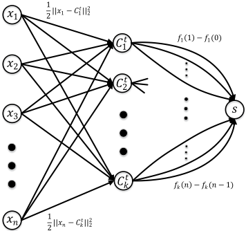
Now, we start to transform problem (10) into an equivalent MCF problem. We construct our flow graph G = (V,A) as follows. Let each data point xi correspond to a vertex which produces one unit flow (bxi = 1). Let each cluster center C th correspond to a transit vertex (bCth = 0). In order to make the problem feasible, we extra add an artificial vertex s with bs = -n. For each pair (xi,C th ), there is an arc from xi to C th with the cost a(xi, C th ) = 1 2 ||xi -C th ||22 . For each center vertex C th , there are n arcs (C th , s)1, (C th , s)2, . . . , (C th , s)n from C th to the artificial vertex s. Let fh be the function associated with cluster h in problem (10). The cost on the ith arc (C th , s)i from C th to s is fh(i) - fh(i - 1). There are no arcs to or from the data point vertex xi to the artificial vertex s. The capacity of each arc in the graph G is 1. Figure 1 illustrates this flow graph. Specifically, we have that
Proposition 1. If all the functions f1, f2, . . . , fk in problem (10) are convex, the minimum cost flow problem defined in (14) is equivalent to problem (10).
Proof. For a solution y of problem (14) and a solution T of problem (10), we use γ(y) and ξ(T ) to denote their objective function values respectively. First, we show that for any solution T of (10), there is a corresponding solution y of (14) with γ(y) + ∑kh=1 fh(0) = ξ(T). Given the solution T of (10), we construct y as follows. For each arc (xi,C th ), let y(xi,C th ) = Ti,h. For the arcs (C th , s)1, . . . , (C th , s)n from vertex C th to vertex s, let y(C th , s)i = 1 for i ≤ nh and y(C th , s)i = 0 for i > nh, where nh = ∑ni=1 Ti,h denotes the number of data points in cluster h. It is easy to verify that y is feasible for (14). In the solution y, the total cost incurred on the arcs (C th , s)1, . . . , (C th , s)n is ∑nh i=1 fh(i) - fh(i - 1) = fh(nh) - fh(0). Thus, we have that γ(y) + ∑kh=1 fh(0) = ξ(T), where ∑kh=1 fh(0) is a constant.
Since bv, v ∈ V and c(u, v), (u, v) ∈ A are all integers, it follows from Proposition 2.3 in [Bertsekas, 1991] that an optimal solution y∗ of the MCF problem (14) is integervalued. Next we show that for any optimal integer-valued solution y∗ of (14), there is a solution T ∗ of (10) with γ(y∗ )+ ∑kh=1 fh(0) = ξ(T ∗ ). Let T ∗ be the solution with T ∗ i,h = 1 if and only if y∗ (xi,C th ) = 1. T ∗ is feasible for (10). Since the functions f1, . . . , fk are convex, the costs on the arcs (C th , s)1, . . . , (C th , s)n are incremental. As y∗ is an optimal solution, one observation is that y∗ (C th , s)i = 1 if i ≤ nh and y∗ (C th , s)i = 0 if i > nh , where nh = ∑ni=1 y∗ (xi,C th ). Thus, we have that γ(y∗ ) + ∑kh=1 fh(0) = ξ(T ∗ ). By the optimality of y∗ , we conclude that T ∗ is optimal for (10).
Proposition 1 provides a method to solve problem (10) by solving an easier equivalent MCF problem when the regularization functions f1, f2, . . . , fk are all convex. Note that the functions defined in (6), (8) and (9) all satisfy the convexity condition.
4.2 Warm Start
Network simplex is a commonly used algorithm for general MCF problems [Bertsekas, 1991]. To solve the proposed model more efficiently, we give an acceleration technique for network simplex and our algorithm regularized k-means (RKM), which is quite useful in practice.
For a linear programming problem, the feasible region defined by all feasible solutions is a (possibly unbounded) convex polytope. An extreme point of the feasible region is a point that is not the midpoint of two other points of the feasible region. In this context an extreme point is also known as a basic feasible solution. It can be shown that for a linear program, if the objective function has an optimal value on the feasible region, then it has this value on (at least) one of the extreme points [Murty, 1983]. It can also be shown that, if an extreme point is not an optimal point of the objective function, then there is an edge of the convex polytope which connects this point to another extreme point with a better objective function value [Murty, 1983]. The simplex algorithm applies this insight by starting at a feasible extreme point and moving along edges of the polytope to extreme points with better and better objective values. Network simplex is a graph theoretic specialization of the general simplex algorithm and works within the same framework.
Going back to our algorithm, it can be seen that the constraints in the MCF problem defined in (14) do not change and only the objective function varies in iterations. In other words, the feasible region of problem (14) is constant, and hence a basic feasible solution at the tth iteration is also a basic feasible solution for the (t+1)th iteration. In practice, we find out that the optimal solution T t+1 i,h of (10) at the (t+1)th Algorithm 1 Regularized k-means with warm start
Input: dataset D, number of desired clusters k and regular-
ization functions f1, f2, . . . , fk
Output: partitioning of dataset
- 1: Randomly initialize center locations C 1 1 , C 1 2 , . . . ,C 1 k .
- 2: y ← a trivial basic feasible solution of problem (14)
- 3: t ← 1
- 4: repeat
- 5: Obtain solution y∗ by solving problem (14) with the start point y.
- 6: Compute new center locations C t+1 1 ,C t+1 2 , . . . ,C t+1 k according to y∗ .
- 7: y ← y∗
- 8: t ← t + 1
- 9: until center locations do not change
- 10: return partitioning corresponding to y
iteration differs little from the solution T t i,h at the tth iteration, when t is large. This phenomenon is reasonable since the cluster centers and the assignment of data points converge gradually in iterations. Instead of solving an MCF problem independently at each iteration, we take the last iteration's solution as the starting extreme point for the current iteration. Compared with starting from a trivial extreme point, it takes much less time for network simplex to find the solution of the current iteration. This technique is called warm start, which combines the advantages of the k-means and simplex methods. The detailed algorithm with warm start is shown in Algorithm 1.
4.3 Convergence
Like the standard k-means, the termination condition of our algorithm is that C th = C t+1 h for h = 1, . . . , k. We end this section by proving a finite convergence result similar to Theorem 7 in [Bradley and Mangasarian, 2000].
Proposition 2. The proposed algorithm regularized k-means (RKM) converges to a solution in a finite number of iterations.
Proof. Consider the objective function (4). At each iteration, the assignment step cannot increase the value of (4). The update step will either strictly decrease the value of (4) or the algorithm terminates since (11) gives the unique optimal solution of (4) when variables Ti,h are fixed to T t i,h . Thus, the value of (4) is strictly decreasing and no repeated clusterings are permitted in iterations. Since there are a finite number of ways to assign n points to k clusters, the algorithm must converge to a solution in a finite number of iterations.
5 Experiments
In a bid to assess the performance of our method regularized k-means (RKM), we compare it with three known balanced clustering algorithms including one soft-balanced and two hard-balanced methods. The soft-balanced algorithm is lasso k-means (LKM) proposed by Li et al. [2018]. It is also a kmeans based algorithm with a specific regularization term in the optimization objective. The two hard-balanced algorithms are the state-of-the-art balanced k-means (BKM) heuristic by Malinen and Fr¨anti [2014] which uses the Hungarian algorithm in the assignment step and the variable neighborhood search based approach "less is more" (LIMA) by Costa et al. [2017]. Specifically, BKM and LIMA both aim to minimize the sum-of-squares under the strict balance constraint: cluster sizes are constrained to ⌊ nk ⌋ or ⌈ nk ⌉, where n is the number of points and k is the number of clusters. We choose these algorithms for comparison due to the common optimization objective: minimizing the imbalance and the sum-of-squares.
5.1 Experiment Setup
Evaluation. We study two performance measures to get a comparative understanding of our method: one is the common optimization objective sum-of-squares used to evaluate the clustering performance and another is the standard deviation in cluster sizes (SDCS) used for the balance evaluation. Let {nh}kh=1 be the sizes of k clusters. SDCS is defined by
Environment and datasets. The source codes of algorithms BKM and LIMA were used in the experiments while LKM was re-implemented in C++ by ourselves. Our method is also implemented in C++. As a platform, Intel Core i78700K 3.70 GHz processor with 16GB memory was used. In the experiments, we consider ten datasets, including six realworld UCI datasets 2 , two artificial datasets s1-s2 3 which have Gaussian clusters with increasing overlap and two MNIST datasets 4 of handwritten digits. The detailed information of the datasets can be found in Table 1. The numbers written under the name of a dataset denote the value of (n, s, k, SDCS), where n refers to the number of points contained in the dataset, s refers to its dimension, k is the number of clusters sought in the dataset and SDCS is computed using the true labels of the dataset.
Regularization settings. To get a contrastive result between our method and LKM, we set the regularization term in our model the same as that in LKM by letting
where λ is the balance parameter. In order to obtain different balancing performance, different values of λ are tested. Specifically, let V ar = ∑ni=1 ||xi-µ||22 where µ = ∑ni=1 xi n be the variance of the dataset {xi}ni=1 , the values of λ are uniformly chosen from the interval [0, 40V ar kn2 ]. For hardbalanced clustering, we use the following functions to derive a strictly balanced result:
for h = 1, . . . , k, where M is a large real number. In the experiments, it is sufficient to set M = V ar.
2 https://archive.ics.uci.edu/ml/index.php
3 http://cs.uef.fi/sipu/datasets/
4 http://yann.lecun.com/exdb/mnist/
| Dataset | Algorithm | Best | Mean | Time |
|---|---|---|---|---|
| Wine | BKM | 2.962e+6 | 2.979e+6 | 3.20e-1 |
| (178, 13, 3, 11.5) | RKM | 2.962e+6 | 2.962e+6 | 2.04e-4 |
| Ionosphere | BKM | 2.434e+3 | 2.435e+3 | 8.08e+0 |
| (351, 34, 2, 70.0) | RKM | 2.434e+3 | 2.434e+3 | 2.81e-4 |
| Libra | BKM | 6.443e+7 | 6.519e+7 | 7.66e+0 |
| (360, 90, 15, 0.0) | RKM | 6.443e+7 | 6.518e+7 | 6.57e-3 |
| User knowledge | BKM | 7.022e+1 | 7.097e+1 | 8.19e+0 |
| (403, 5, 4, 39.5) | RKM | 7.021e+1 | 7.096e+1 | 1.31e-3 |
| Vowel recognition | BKM | 3.314e+7 | 3.320e+7 | 9.68e+1 |
| (871, 3, 6, 53.5) | RKM | 3.314e+7 | 3.314e+7 | 8.08e-3 |
| Multiple features | BKM | 1.784e+6 | (one run) | 1.20e+3 |
| (2000, 240, 10, 0.0) | RKM | 1.750e+6 | 1.758e+6 | 1.87e-1 |
| s1 | BKM | 1.095e+13 | (one run) | 7.67e+3 |
| (5000, 2, 15, 16.0) | RKM | 1.089e+13 | 1.089e+13 | 4.56e-1 |
| s2 | BKM | 1.431e+13 | (one run) | 5.24e+3 |
| (5000, 2, 15, 15.8) | RKM | 1.428e+13 | 1.428e+13 | 4.62e-1 |
| MNIST-test | BKM | - | - | > 1 day |
| (10000, 784, 10, 62.4) | RKM | 2.542e+10 | 2.546e+10 | 4.35e+0 |
| MNIST-train | BKM | - | - | > 1 day |
| (60000, 784, 10, 340.0) | RKM | 1.536e+11 | 1.536e+11 | 3.17e+1 |
5.2 Experiment Results
The effect of the balance parameter λ on the clustering and balancing performance of LKM and our algorithm RKM are demonstrated in Figure 2, where we take four representative datasets as examples. In Figure 2, a point is obtained by 100 executions of LKM or RKM with random initial solutions and the corresponding value of λ. The mean of sum-ofsquares (SDCS respectively) of these 100 executions is shown on the vertical axis. Table 1 gives the comparison results of BKM and RKM. Column Best and Mean refer to the best sum-of-squares value and the mean sum-of-squares value respectively, obtained from 100 runs. Both BKM and RKM start from the same random initial solutions, which are made distinct in each execution. The last column (Time) presents the average CPU time (in sec) used in each run. Finally, the comparisons of LIMA and RKM are shown in Table 2. Since LIMA is a neighborhood search based heuristic, the more computing time is given, the better solution it finds. We compare our algorithm with LIMA in different running time limits. The best sum-of-squares value found in 100 executions of our algorithm is reported in column RKM. T RKM is the average CPU time (in sec) used in each execution of our algorithm. The column LIMA k× gives the best solution value found in 100 executions of LIMA, with a running time limit k×T RKM for each execution. According to the experiment results, we have the following observations:
| Dataset | RKM | T RKM | LIMA 1× | LIMA 100× |
|---|---|---|---|---|
| Wine | 2.962e+6 | 2.04e-4 | 2.973e+6 | 2.962e+6 |
| Ionosphere | 2.434e+3 | 2.81e-4 | 2.467e+3 | 2.434e+3 |
| Libra | 6.443e+7 | 6.57e-3 | 6.468e+7 | 6.394e+7 |
| User knowledge | 7.021e+1 | 1.31e-3 | 7.536e+1 | 7.033e+1 |
| Vowel recognition | 3.314e+7 | 8.08e-3 | 2.616e+08 | 7.652e+07 |
| Multiple features | 1.750e+6 | 1.87e-1 | 2.582e+06 | 1.782e+06 |
| s1 | 1.089e+13 | 4.56e-1 | 5.593e+14 | 4.776e+13 |
| s2 | 1.428e+13 | 4.62e-1 | 4.984e+14 | 3.752e+13 |
| MNIST-test | 2.542e+10 | 4.35e+0 | 2.834e+10 | 2.543e+10 |
| MNIST-train | 1.536e+11 | 3.17e+1 | MEM> 16G | MEM> 16G |
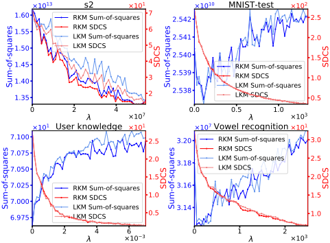
- In the experiments of soft-balanced clustering, our algorithm RKM shares the same objective function with LKM but they differ in the optimization methods. We can see that RKM and LKM show similar balancing performance while RKM outperforms LKM in clustering performance, especially for highly balanced clustering.
- There is an obvious positive correlation between the balancing performance and the balance parameter λ for both algorithms LKM and RKM. However, the effect of λ on the objective function sum-of-squares is not consistent. It depends on the type of data. For example, the data points in s2 have a balanced distribution, so a larger value of λ may derive a better solution. It also indicates that the balance regularization may be beneficial to avoid poor local minima for the standard k-means algorithm.
- Thanks to the efficiency of network simplex and the warm start technique, our algorithm is several orders of magnitude faster than the balanced k-means (BKM) algorithm. Due to the space limitation, the effect of warm start is not demonstrated. Roughly speaking, it gives a 7 to 18 times speedup for RKM on large datasets.
- In order to get better solutions, one way is to execute RKM many times starting from different initial solutions. Compared with the neighborhood search based heuristic LIMA, RKM can give a better solution within less time on most datasets except Libra.
Acknowledgements
This work was supported by the National Natural Science Foundation of China, under grants 61772115 and 61370071.
@inproceedings{ijcai2019p414,
  title     = {Balanced Clustering: A Uniform Model and Fast Algorithm},
  author    = {Lin, Weibo and He, Zhu and Xiao, Mingyu},
  booktitle = {Proceedings of the Twenty-Eighth International Joint Conference on
               Artificial Intelligence, {IJCAI-19}},
  publisher = {International Joint Conferences on Artificial Intelligence Organization},
  editor    = {Sarit Kraus},
  pages     = {2987--2993},
  year      = {2019},
  month     = {8},
  note      = {Main track},
  doi       = {10.24963/ijcai.2019/414},
  url       = {https://doi.org/10.24963/ijcai.2019/414},
}
TY - CPAPER TI - Balanced Clustering: A Uniform Model and Fast Algorithm AU - Lin, Weibo AU - He, Zhu AU - Xiao, Mingyu T2 - Proceedings of the Twenty-Eighth International Joint Conference on Artificial Intelligence, IJCAI-19 PB - International Joint Conferences on Artificial Intelligence Organization PY - 2019 SP - 2987 EP - 2993 DO - 10.24963/ijcai.2019/414 UR - https://doi.org/10.24963/ijcai.2019/414 ER -Copied
Machine-readable versions of this paper, for tools and AI agents:





