
Learning Low-precision Neural Networks without Straight-Through Estimator (STE)
Proceedings of the Twenty-Eighth International Joint Conference on Artificial Intelligence. Main track. Pages 3066-3072.
https://doi.org/10.24963/ijcai.2019/425
Keywords
- Machine Learning: Classification
- Machine Learning: Deep Learning
Abstract
The Straight-Through Estimator (STE) is widely used for back-propagating gradients through the quantization function, but the STE technique lacks a complete theoretical understanding. We propose an alternative methodology called alpha-blending (AB), which quantizes neural networks to low precision using stochastic gradient descent (SGD). Our AB method avoids STE approximation by replacing the quantized weight in the loss function by an affine combination of the quantized weight w_q and the corresponding full-precision weight w with non-trainable scalar coefficient alpha and (1- alpha). During training, alpha is gradually increased from 0 to 1; the gradient updates to the weights are through the full precision term, (1-alpha) * w, of the affine combination; the model is converted from full-precision to low precision progressively. To evaluate the AB method, a 1-bit BinaryNet on CIFAR10 dataset and 8-bits, 4-bits MobileNet v1, ResNet_50 v1/2 on ImageNet are trained using the alpha-blending approach, and the evaluation indicates that AB improves top-1 accuracy by 0.9\%, 0.82\% and 2.93\% respectively compared to the results of STE based quantization.
- [Bengio et al., 2013] Yoshua Bengio, Nicholas Léonard, and Aaron C. Courville. Estimating or propagating gradients through stochastic neurons for conditional computation. CoRR, abs/1308.3432, 2013.
- [Courbariaux et al., 2015] Matthieu Courbariaux, Yoshua Bengio, and Jean-Pierre David. Binaryconnect: Training deep neural networks with binary weights during propaga- tions. CoRR, abs/1511.00363, 2015.
- [Dally, 2015] William Dally. Nips tutorial 2015. https://media.nips.cc/Conferences/2015/tutorialslides/Dally- NIPS-Tutorial-2015.pdf, 2015. Link
- [Goetschalckx et al., 2018] Koen Goetschalckx, Bert Moons, Patrick Wambacq, and Marian Verhelst. Effi- ciently combining svd, pruning, clustering and retraining for enhanced neural network compression. pages 1-6, 06 2018.
- [Han et al., 2015] Song Han, Huizi Mao, and William J. Dally. Deep compression: Compressing deep neural net- work with pruning, trained quantization and huffman cod- ing. CoRR, abs/1510.00149, 2015.
- [Hinton et al., 2012] Geoffrey Hinton, li Deng, Dong Yu, George E. Dahl, Abdel-rahman Mohamed, Navdeep Jaitly, Andrew Senior, Vincent Vanhoucke, Phuongtrang Nguyen, Tara Sainath, and Brian Kingsbury. Deep neural networks for acoustic modeling in speech recognition: The shared views of four research groups. Signal Processing Magazine, IEEE, 29:82-97, 11 2012.
- [Hinton, 2012] G. Hinton. Neural networks for machine learning, 2012.
- [Howard et al., 2017a] Andrew G. Howard, Menglong Zhu, Bo Chen, Dmitry Kalenichenko, Weijun Wang, Tobias Weyand, Marco Andreetto, and Hartwig Adam. Mo- bilenets: Efficient convolutional neural networks for mo- bile vision applications. CoRR, abs/1704.04861, 2017.
- [Howard et al., 2017b] Andrew G. Howard, Menglong Zhu, Bo Chen, Dmitry Kalenichenko, Weijun Wang, Tobias Weyand, Marco Andreetto, and Hartwig Adam. Mo- bilenets: Efficient convolutional neural networks for mo- bile vision applications. CoRR, abs/1704.04861, 2017.
- [Hubara et al., 2016a] Itay Hubara, Matthieu Courbariaux, Daniel Soudry, Ran El-Yaniv, and Yoshua Bengio. Bina- rized neural networks. In D. D. Lee, M. Sugiyama, U. V. Luxburg, I. Guyon, and R. Garnett, editors, Advances in Neural Information Processing Systems 29, pages 4107- 4115.
- Curran Associates, Inc., 2016.
- [Hubara et al., 2016b] Itay Hubara, Daniel Soudry, and Ran El Yaniv. Binarized neural networks. CoRR, abs/1602.02505, 2016. Withdrawn.
- [Iandola et al., 2016] Forrest N. Iandola, Matthew W. Moskewicz, Khalid Ashraf, Song Han, William J. Dally, and Kurt Keutzer. Squeezenet: Alexnet-level accuracy with 50x fewer parameters and <1mb model size. CoRR, abs/1602.07360, 2016.
- [Krishnamoorthi, 2018] Raghuraman Krishnamoorthi. Quantizing deep convolutional networks for efficient inference: A whitepaper. CoRR, abs/1806.08342, 2018.
- [Krizhevsky et al., 2017] Alex Krizhevsky, Ilya Sutskever, and Geoffrey E. Hinton. Imagenet classification with deep convolutional neural networks. Commun. ACM, 60(6):84- 90, May 2017.
- [Leng et al., 2017] Cong Leng, Hao Li, Shenghuo Zhu, and Rong Jin. Extremely low bit neural network: Squeeze the last bit out with ADMM. CoRR, abs/1707.09870, 2017.
- [Li and Liu, 2016] Fengfu Li and Bin Liu. Ternary weight networks. CoRR, abs/1605.04711, 2016.
- [Penghang Yin, 2018] Shuai Zhang Stanley Osher Yingyong Qi Jack Xin Penghang Yin, Jiancheng Lyu. Understanding straight-through estimator in training activation quantized neural nets. 2018.
- [Rastegari et al., 2016a] Mohammad Rastegari, Vicente Or- donez, Joseph Redmon, and Ali Farhadi. Xnor-net: Ima- genet classification using binary convolutional neural net- works. CoRR, abs/1603.05279, 2016.
- [Rastegari et al., 2016b] Mohammad Rastegari, Vicente Or- donez, Joseph Redmon, and Ali Farhadi. Xnor-net: Ima- genet classification using binary convolutional neural net- works. CoRR, abs/1603.05279, 2016.
- [Rastegari et al., 2016c] Mohammad Rastegari, Vicente Or- donez, Joseph Redmon, and Ali Farhadi. Xnor-net: Ima- genet classification using binary convolutional neural net- works. CoRR, abs/1603.05279, 2016.
- [Xue et al., 2013] J Xue, J Li, and Y Gong. Restructuring of deep neural network acoustic models with singular value decomposition. Proceedings of the Annual Conference of the International Speech Communication Association, IN- TERSPEECH, pages 2365-2369, 01 2013.
- [Yin et al., 2018] Penghang Yin, Shuai Zhang, Jiancheng Lyu, Stanley Osher, Yingyong Qi, and Jack Xin. Blended Coarse Gradient Descent for Full Quantization of Deep Neural Networks. arXiv e-prints, page arXiv:1808.05240, Aug 2018.
- [Zhou et al., 2017] Aojun Zhou, Anbang Yao, Yiwen Guo, Lin Xu, and Yurong Chen. Incremental network quanti- zation: Towards lossless cnns with low-precision weights. CoRR, abs/1702.03044, 2017.
References were extracted automatically from the PDF and may contain errors.
Full text extracted automatically from the PDF; figures, tables and equations may differ. The PDF is the version of record.
1 Introduction
Deep Neural Networks (DNNs) have demonstrated outstanding performance on a wide range of tasks, including image classification [Krizhevsky et al., 2017], speech recognition [Hinton et al., 2012] etc. These networks typically consists of multiple convolution layers with a large number of parameters. The models are trained on high performance servers typically with GPUs and are deployed on lower-end machines, i.e. mobile or IoT devices, for inference tasks. Improved inference accuracy usually comes with millions of model parameters and high computation cost. For example, the largest Mobilenet v1 model [Howard et al., 2017a] has 4.2 million parameters and 569 million floating point MAC per inference 1 . For applications that demand high inference accuracy, low latency and low power consumption, the large memory requirements and computation costs are a significant challenge for constrained platforms.
1 https://github.com/tensorflow/models/blob/master/research/ slim/nets/mobilenet v1.md
2 https://github.com/tensorflow/models/tree/master/research/slim
To achieve efficient inference, one approach is to design compact network architectures from scratch [Howard et al., 2017b] [Iandola et al., 2016] [Rastegari et al., 2016a] [Li and Liu, 2016]. Alternatively, existing models can be optimized for efficiency. There are several optimization techniques that boost efficiency when applied to pretrained models: weight pruning [Han et al., 2015] [Goetschalckx et al., 2018], weight clustering [Han et al., 2015] [Goetschalckx et al., 2018], singular value decomposition (SVD) [Xue et al., 2013] and quantization [Courbariaux et al., 2015] [Rastegari et al., 2016b] [Zhou et al., 2017]. The basic principle is to reduce the number of parameters and/or lower the computation cost of inference. Weight pruning techniques remove parameters while minimizing the impact on inference accuracy. Weight clustering clusters similar weights to shrink the overall size of a model. The SVD method potentially reduces both model size and computation cost through discarding small singular values. Quantization techniques 3 4 5 convert normal floating-point values to narrow and cheaper integer or fixed point i.e. 8-bits, 4-bits or binary multiplication operations without incurring significant loss in the accuracy. There are three major benefits to quantization: reduced memory bandwidth, reduced memory storage, and higher throughput computation. The predominant numerical format used for training neural networks is IEEE fp32 format. There is a potential 4x reduction in overall bandwidth and storage if one can quantize fp32 floating point to 8-bits for both weight and activation. The corresponding energy and area saving are 18x and 27x [Dally, 2015] respectively. The efficient computation kernel libraries for fast inference, i.e. ArmCMSIS 6 , Gemmlowp 7 , Intel MKL-DNN 8 , Nvidia TensorRT 9 and custom ASIC hardware, are built upon the reduced precision numerical forms.
3 https://petewarden.com/2015/05/23/ why-are-eight-bits-enough-for-deep-neural-networks
4 https://petewarden.com/2016/05/03/ how-to-quantize-neural-networks-with-tensorflow
5 https://petewarden.com/2017/06/22/
what-ive-learned-about-neural-network-quantization 6 http://arm-software.github.io/CMSIS5/NN/html/index.html
The Straight-Through Estimator (STE) [Hinton, 2012][Bengio et al., 2013] is widely implemented in discrete optimization using SGD due to its effectiveness and simplicity. STE is an empirical workaround to the gradient vanishing issue in Backprop; however it lacks complete mathematical justification especially for large-scale optimization problems [Penghang Yin, 2018]. In this paper, we propose a novel optimization technique, termed alpha-blending (AB), for quantizing full precision networks to lower precision representations(8-bits, 4-bits or 1-bit). AB does not rely on the concept of STE to back-propagate the gradient update to weights; AB instead replaces the weight vector w in the loss function by the expression wab = (1 - α)w + αwq, which is the affine combination of the w and its quantization wq. During training, we gradually increase the non-trainable parameter α from 0.0 to 1.0. This formulation isolates the quantized weights wq from the full-precision trainable weights w and therefore avoids the challenges arising from the use of Straight-Through Estimation (STE).
To evaluate the performance of the proposed method, we trained single-bit BinaryNet [Hubara et al., 2016a] on CIFAR10 and 4-bits, 8-bits MobileNet v1, ResNet v1 and v2 models on the ImageNet dataset. AB outperforms previous state-of-art STE based quantization 0.9% for 1-bit BinaryNet and 2.9% for 4-bits weight and 8-bits activation (4-8) [Krishnamoorthi, 2018] in top-1 accuracy. Moreover, we have applied our AB approach to quantize MobileNet v1, ResNet v1,2 networks with both 4-bit weight as well as 4-bit activation (4b/4b). In this configuration, our 4b/4b quantization delivers similar accuracy level as the best known 4b/8b quantization approach [Krishnamoorthi, 2018].
2 RelatedWorks
There is a significant body of research on neural network quantization techniques from the deep learning community. BinaryConnect [Courbariaux et al., 2015] binarizes the weights of neural networks using the sign function. Binary Weight Network [Rastegari et al., 2016c] has the same binarization while introducing a scaling factor. BinaryNet [Hubara et al., 2016b] [Hubara et al., 2016a] quantizes both weights and activations to binary values. TWN [Li and Liu, 2016] constructs networks with ternary values 0, +/-1 to balance the accuracy and model compression compared to the binary quantization. STE [Hinton, 2012] is used to approximate the gradient of quantization function during the learning process. Once they are quantized, these models eliminate majority of the floating-point multiplications, and therefore exhibit improved power efficiency by using SIMD instructions on commodity micro-processor or via special hardware. On the downside, the single bit quantization schemes often lead to substantial accuracy drop on large scale dataset while achieving good results on simple dataset such as MNIST, CIFAR10.
7 https://github.com/google/gemmlowp
8 https://intel.github.io/mkl-dnn/index.html
9 http://on-demand.gputechconf.com/gtc/2017/presentation/ s7310-8-bit-inference-with-tensorrt.pdf
Another approach is to train the network in full floatingpoint domain, then statically quantize the model parameter into reduced numerical forms and keep the activation in floating-point. Googles Tensorflow provides a post-training quantization flow 10 to convert float-point weights into 8-bits of precision from INT8. Its uniform affine quantization maps a set of floating-point values to 8-bits unsigned integers by shifting and scaling [Krishnamoorthi, 2018]. The minimum and maximum values correspond to quantized value 0 and 255 respectively. Another mapping scheme is uniform symmetric quantizer, which scales the maximum magnitude of floating-point values to maximum 8-bit integer e.g. 127 and the floating-point zero always mapped to quantized zero. The conversion is done once, and reduction of model size is up to 4X. A further improvement dynamically quantizes activations into 8-bits as well at inference. With 8-bits weight and activation, one can switch the most compute-intensive operations e.g. convolution, matrix multiply (GEMM) from original floating-point format to the cheaper operation, and reduces the latency as well.
The main drawback of such post-processing approach is the degradation in model accuracy. To overcome this accuracy drop, quantization aware training 11 techniques have been developed to ensure that the forward pass uses the reduced precision for both training and inference. To achieve this, full precision weights and activations values flow through fake quantization nodes, then quantized values feed through convolution or matrix multiply. Applying the Straight-Through Estimator (STE) approximation [Hinton, 2012] [Hubara et al., 2016a] [Yin et al., 2018], the operations in the back propagation phase are still at full precision as this is required to provide sufficient precision in accumulating small adjustment to the parameters.
3 Alpha-blending, the ProposedMethod (AB)
We introduce an optimization methodology, alpha-blending (AB), for quantizing neural networks. Section 3.1 describes the scheme of AB and weights quantization; section 3.2 sketches the quantization of activation using AB.
3.1 Quantization of Weights
During quantization-aware training, the full precision weights are quantized to low precision values wq . Mathematically, we want to minimize a convex function L(w) as equation 1 with the additional constraint that w must be n-bit signed integers i.e. w ∈ Q = [-(2n-1 - 1), 2n-1 - 1].
Previous approaches i.e. 11 , [Hubara et al., 2016a] insert quantizer nodes in the computation graph. These nodes receive full precision input w and generate quantized output wq = q(w), between the full precision weights w and computation nodes as in Figure 1. The quantized weights wq = q(w) are used in the forward and backward pass while the gradient update to the full precision weight uses full precision to ensure smooth updates to the weights. But the quantization function has zero gradient almost everywhere ∂wq/∂w = a.e. 0, which prevents further backpropagation of gradients and halts learning. The Straight-Through Estimator (STE) [Hinton, 2012] [Hubara et al., 2016a] [Krishnamoorthi, 2018] was developed to avoid the vanishing gradient problem illustrated in Figure 1. STE approximates quantization with the identity function I(w) = w in Backprop as eq. 2. Therefore with STE, the gradient of the quantization function with respect to the full precision weight is approximated using the quantized weight as in equation 3. We hypothesize that the error introduced by this approximation may impact the accuracy of the gradient computation, thereby degrading overall network accuracy, especially for very low precision (1-bit or 4-bit) networks.∂wq
10 https://www.tensorflow.org/lite/performance/post training quantization
11 https://github.com/tensorflow/tensorflow/tree/master/ tensorflow/contrib/quantize
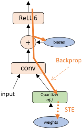
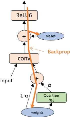
Our proposed method, alpha-blending (AB), does not rely on the Straight-Through Estimator (STE) to overcome the quantizer's vanishing gradient problem in Backprop, therefore it eliminates the quantization error due to equation 3. AB replaces the weight term in the loss function by (1 - α)w + αwq, an affine combination of the original full precision weight term and its quantized version with coefficient α. The new loss function Lab(w, α) for a neural network is shown in equation 4. The gradient of Lab(w, α) with respect to the weights is in equation 5, accepting the zero gradient of quantization function ∂wq/∂w = a.e. 0 without STE approximation. Its Backprop flow is illustrated in figure 2.
Figure 2: AB quantization performs the convolution using an affine combination of the full precision weights and the quantized weights. The coefficient α is gradually increased from 0 to 1 during training. This approach avoids back-propagation through the Quantizer, eliminating the gradient vanishing path (from the quantized weight node in light green to the weight node in blue). There is no need to apply Straight Trough Estimator (STE) during the Backprop. The actual weight gradient update goes through the (1 - α) path, where the gradient, eq. 5, is well-defined.
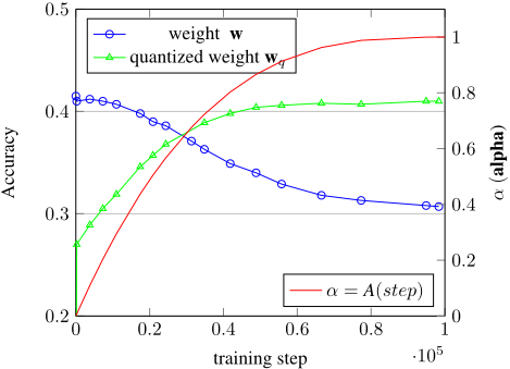
The AB flow gradually increases the non-trainable parameter α from 0 to 1 using a function of the form shown in equation 6 for training steps in the optimization window [T0, T1]. An example is shown in Figure 4. The function in equation 6 is not unique, for example, an alternative choice is A(step, λ) = 1 - e-λ·step . The optimization window [T0, T1], during which α is increased, is a user-defined hyper parameter.
We use algorithm 2 described in section 4.2 to convert w to wq = γw · qw , where γw is a scaling factor and qw ∈ Q, at certain frequency, quantizing frequency, in training steps.
Algorithm 1 summarizes the AB optimization procedure, in
Algorithm 1 Alpha-blending optimization (ABO)
Input: derivative loss function L(w) Def. function: Lab(w,wq, α) = L((1 -α)w+αwq) Initialize: w ← w0, α ← 0, ε ← learning rate, f ← optimization frequency, T0, T1 ← traing window for step = 0 to T do wq ← Algorithm 2 PPQ(w) or other optimization function (w) w←w- ε · (1-α) ∂L(w′ ) ∂w′ ∣∣∣∣w′ =(1-α)w+αwq if step % f = 0 and α < 1 then α←A(step) {Raising α toward to 1.0; eq 6}
end if end for Output: wq
which the original learning rate ε is scaled by the factor (1 - α) to act as an effective learning rate ε · (1 - α).
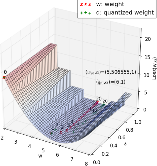
To visualize the process, figure 3 demonstrates how to solve the trivial example, arg min s.t. w∈Q (w - 5.7)2 = 6 using AB.
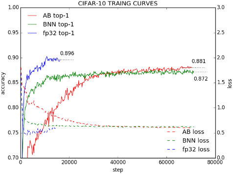
To compare the AB optimization concept with STE, we trained the single bit 8-layer BinaryNet defined in [Hubara et al., 2016a] on the CIFAR10 dataset in section 4.1, figure 5. The top-1 accuracy score achieved with AB is 0.9% higher compared to the accuracy achieved with STE. Figure 4 shows a more practical example of AB quantization using MobileNet 1.0 0.25/128 v1 on the ImageNet dataset. The AB quantization flow gradually transforms the full precision model at α = 0 to a model with quantized weights wq at α = 1.0 with an accuracy loss of 0.6% versus the full precision model.
3.2 Quantization of Activation
AB uses the PPQ, algorithm 2 in section 4.2, to quantize the input feature maps or activation a to aq as well, and accumulates the scaling factor γa via exponential moving average with the smoothing parameter being close to 1, e.g. 0.99. Thus a can be approximated as a ≈ γa · qa
For inference (α=1), the floating point computation of the kth layer in forward pass is a(k+1) = δ(w(k) a(k) +b(k) ). With the quantizaton of both weight and activation, the same calculation becomes eq. 7.
(qw · qa ) in 7 is the compute-intensive operation of matrix multiply or convolution (GEMM) in low precision quantized values, which will gain significant power efficiency compared to the original floating-point version. Other relatively unimportant terms in 7 e.g. (γwγa) and b can be represented by higher precision fixed points.
4 Experiments
To evaluate the AB quantization methodology, we performed several experiments. The first one, in section 4.1, is a single bit (1-bit) control test between STE and AB on CIFAR10. Section 4.2 presents results for Mobilenet v1 and ResNet v1,2 with the ImageNet ILSVRC 2012 dataset. All evaluations were performed on a x86 64 ubuntu Linux based Xeon server, Lenovo P710, with a TitanV GPU.
4.1 BinaryNet with Alpha-blending (AB)
To evaluate AB's function directly, 1-bit BinaryNet (BNN) 12 [Hubara et al., 2016a] on CIFAR-10 was trained on Tensorflow using AB and STE respectively. Both weight and activation are quantized into +1 or -1 (single bit) by the same binarization function, binarize(x) = Sign(x). Figure 5 shows the results of these experiments. The AB method achieves a top-1 accuracy of 88.1%. Using STE, we achieve 87.2%. The FP32 baseline accuracy is 89.6%.
4.2 4-bits and 8-bits Quantization withMobileNet and ResNet
In this section, we describe the iterative quantization scheme we use to quantize FP32 values to low-precision, Progressive Projection Quantization (PPQ). We apply PPQ to convert floating point values into 4-bits or 8-bits integers, then utilize PPQ and AB to quantize MobileNet and ResNet into 4-bits or 8-bits and compare the result with existing results.
Progressive Projection Quantization, PPQ
To quantize a set of N floating-point values x = {xi|i ∈ [0,N - 1]} to symmetric n-bits signed integer set xq = {qi | qi ∈ Q = (0,±1,±2, ...,±(2n-1 -1)), i ∈ [0,N - 1]} with a positive scaling factor γ, we can approximate the initial quantization by rounding xi γ ∣∣∣γ= max|x| 2n-1-1 to the nearest-
neighbor in Q as equation 8. Then we can improve γ by equation 9.
PPQ is an iterative procedure: by repeatedly applying eq. 8 and 9, as described in algorithm 2, projects vector x onto space Q to determine γ progressively [Leng et al., 2017]. The procedure is guaranteed to converge to a local minimum. In practice, convergence is very fast and 3 iterations is enough. Thus, x can be approximated by the product of the scalar γ and xq: x ≈ γxq = γ · round( xγ )
INT8-8: Evaluation of 8-bits Weight and Activation
The top-1 accuracy for 8-bit weight and 8-bit activation quantization are listed in table 1. The 2nd column gives the fp32 accuracy of the pre-trained models 1 . The 3rd column contains the quantization results 1 2 . The last column gives the best results that AB generated. Both quantization approaches delivered roughly the same top-1 accuracy, although AB has slightly (0.82%) better accuracy on average.
12 https://github.com/itayhubara/BinaryNet.tf
Algorithm 2 Progressive Project Quantization (PPQ)
Input: full precision vector x = {xi|i ∈ [0,N - 1]},
scaling factor γ
if γ ≤ 0 then
end if
repeat
end for
γ ← 〈x,q〉
〈q,q〉
until γ = γ0
Output: q, γ
INT4-8: Evaluation of 4-bits Weight and 8-bits Activation
[Krishnamoorthi, 2018] reported that accuracy of 4-bits weight and 8-bits activation (INT4-8) is within 5% of the fp32 baseline for Mobilenet v1 and ResNet networks. We ran the same models using AB quantization, and have listed the result in the 4th and 5th columns in table 2. The 4th one is per-layer quantization, and 5th is per-channel. AB INT4-
| Model name | fp32 % | TF8-8 % | AB8-8 % |
|---|---|---|---|
| MB 1.0 224v1 | 70.9 | 70.1 | 70.9 |
| MB 1.0 128v1 | 65.2 | 63.4 | 65.0 |
| MB 0.75 224v1 | 68.4 | 67.9 | 68.2 |
| MB 0.75 128v1 | 62.1 | 59.8 | 61.6 |
| MB 0.5 224v1 | 63.3 | 62.2 | 63.0 |
| MB 0.5 128v1 | 56.3 | 54.5 | 55.8 |
| MB 0.25 224v1 | 49.8 | 48 | 49.2 |
| MB 0.25 128v1 | 41.5 | 39.5 | 40.9 |
| ResNet 50v1 | 75.2 | 75∗ | 75.1 |
| ResNet 50v2 | 75.6 | 75∗ | 75.4 |
8 achieved a 1.53% accuracy drop on average compared to the fp32 baseline for per-layer quantization, and a 0.9% accuracy drop for per-channel quantization. Moreover, AB's INT4-8 per-channel performance outperforms the prior result [Krishnamoorthi, 2018] in 3rd col. by 2.93%.
INT4-4: Evaluation of 4-bits Weight and 4-bits Activation
Finally, we quantized the well-known neural networks, MobileNet 1.0 224 v1 and ResNet 50 v1/v2, using 4-bit weights and 4-bit activations. The 4th column in table 3 is for perlayer quantization, whose accuracy is 5.5% lower than fp32's in average. The per-channel quantization in the 5th column has 4.66% accuracy loss. AB's INT4-4 result, using perchannel quantization, achieves similar accuracy as the TF4-8
| Model name | fp32 % | TF4-8 % | AB4-8 per-layer % | AB4-8 per-channel % |
|---|---|---|---|---|
| MB1.0 224v1 | 70.9 | 65.0+ | 68.7 | 69.6 |
| MB0.75 224v1 | 68.4 | - | 65 | - |
| MB0.50 224v1 | 63.3 | - | 58.4 | - |
| MB0.25 224v1 | 49.8 | - | 43.8 | - |
| ResNet 50v1 | 75.2 | 73.2+ | 73.8 | 74.3 |
| ResNet 50v2 | 75.6 | 72+ | 74.6 | 75.1 |
| Model name | fp32 % | TF4-8 % | AB4-4 per-layer % | AB4-4 per-channel % |
|---|---|---|---|---|
| MB1.0 224v1 | 70.9 | 65.0+ | 61.8 | 64.3 |
| ResNet 50v1 | 75.2 | 73.2+ | 69.6 | 71.2 |
| ResNet 50v2 | 75.6 | 72+ | 71.6 | 72.2 |
scheme [Krishnamoorthi, 2018], which has 4-bits weight and 8-bits activation as shown in the 3rd column.
5 Conclusion and FutureWork
We have introduced alpha-blending (AB), an alternative method to the well-known Straight-Through Estimator (STE) for learning low precision neural networks using SGD. AB accepts the almost everywhere zero gradient of quantization function during Backprop, and uses an affine combination of the original full-precision weights and corresponding quantized values as the actual weights in the loss function. This change allows the gradient update to the full-precision weights in backward propagation to be performed through the full-precision path incrementally, instead of applying STE to the quantization path.
To measure the impact on network accuracy using the AB methodology, we have trained a single-bit BinaryNet(BBN) [Hubara et al., 2016a] on CIFAR10 to show that AB generates equivalent or better accuracy compared to training with STE. Moreover, we have applied the AB metholody to larger, more practical networks such as MobileNet and ResNet to compare with STE based quantization. The top-1 accuracy of 8-bits weight and 8-bits activation is 0.82% better than the existing state-of-art results 1 2 . For 4-bits weight and 8-bits activation quantization, AB has 2.93% higher top-1 accuracy on average compared to that reported in [Krishnamoorthi, 2018].
AB can also be applied to several other network optimization techniques besides quantization. We plan to investigate AB on clustering and pruning in a future work.
@inproceedings{ijcai2019p425,
  title     = {Learning Low-precision Neural Networks without Straight-Through Estimator (STE)},
  author    = {Liu, Zhi-Gang and Mattina, Matthew},
  booktitle = {Proceedings of the Twenty-Eighth International Joint Conference on
               Artificial Intelligence, {IJCAI-19}},
  publisher = {International Joint Conferences on Artificial Intelligence Organization},
  editor    = {Sarit Kraus},
  pages     = {3066--3072},
  year      = {2019},
  month     = {8},
  note      = {Main track},
  doi       = {10.24963/ijcai.2019/425},
  url       = {https://doi.org/10.24963/ijcai.2019/425},
}
TY - CPAPER TI - Learning Low-precision Neural Networks without Straight-Through Estimator (STE) AU - Liu, Zhi-Gang AU - Mattina, Matthew T2 - Proceedings of the Twenty-Eighth International Joint Conference on Artificial Intelligence, IJCAI-19 PB - International Joint Conferences on Artificial Intelligence Organization PY - 2019 SP - 3066 EP - 3072 DO - 10.24963/ijcai.2019/425 UR - https://doi.org/10.24963/ijcai.2019/425 ER -Copied
Machine-readable versions of this paper, for tools and AI agents:





