
Gradient Boosting with Piece-Wise Linear Regression Trees
Proceedings of the Twenty-Eighth International Joint Conference on Artificial Intelligence. Main track. Pages 3432-3438.
https://doi.org/10.24963/ijcai.2019/476
Keywords
- Machine Learning: Ensemble Methods
- Machine Learning: Classification
Abstract
Gradient Boosted Decision Trees (GBDT) is a very successful ensemble learning algorithm widely used across a variety of applications. Recently, several variants of GBDT training algorithms and implementations have been designed and heavily optimized in some very popular open sourced toolkits including XGBoost, LightGBM and CatBoost.
In this paper, we show that both the accuracy and efficiency of GBDT can be further enhanced by using more complex base learners. Specifically, we extend gradient boosting to use piecewise linear regression trees (PL Trees), instead of piecewise constant regression trees, as base learners. We show that PL Trees can accelerate convergence of GBDT and improve the accuracy. We also propose some optimization tricks to substantially reduce the training time of PL Trees, with little sacrifice of accuracy. Moreover, we propose several implementation techniques to speedup our algorithm on modern computer architectures with powerful Single Instruction Multiple Data (SIMD) parallelism. The experimental results show that GBDT with PL Trees can provide very competitive testing accuracy with comparable or less training time.
- [Breiman, 2017] Leo Breiman. Classification and Regres- sion Trees. Routledge, 2017.
- [Chen and Guestrin, 2016] Tianqi Chen and Carlos Guestrin. XGBoost: A scalable tree boosting system. In Proceedings of the 22nd ACM SIGKDD International Conference on Knowledge Discovery and Data Mining, pages 785-794. ACM, 2016.
- [Chen et al., 2012] Tianqi Chen, Linpeng Tang, Qin Liu, Diyi Yang, Saining Xie, Xuezhi Cao, Chunyang Wu, En- peng Yao, Zhengyang Liu, Zhansheng Jiang, et al. Com- bining factorization model and additive forest for collabo- rative followee recommendation. KDD CUP, 2012.
- [Dobra and Gehrke, 2002] Alin Dobra and Johannes Gehrke. Secret: a scalable linear regression tree algorithm. In Pro- ceedings of the 8th ACM SIGKDD International Confer- ence on Knowledge Discovery and Data Mining, pages 481-487. ACM, 2002.
- [Espasa et al., 1998] Roger Espasa, Mateo Valero, and James E Smith. Vector architectures: past, present and fu- ture. In Proceedings of the 12th International Conference on Supercomputing, pages 425-432. ACM, 1998.
- [Friedman et al., 2000] Jerome Friedman, Trevor Hastie, Robert Tibshirani, et al. Additive logistic regression: a sta- tistical view of boosting (with discussion and a rejoinder by the authors). The Annals of Statistics, 28(2):337-407, 2000.
- [Friedman, 1979] Jerome H Friedman. A tree-structured ap- proach to nonparametric multiple regression. Smoothing Techniques for Curve Estimation, 757:5-22, 1979.
- [Friedman, 2001] Jerome H Friedman. Greedy function ap- proximation: a gradient boosting machine. Annals of Statistics, pages 1189-1232, 2001.
- [Hall et al., 2009] Mark Hall, Eibe Frank, Geoffrey Holmes, Bernhard Pfahringer, Peter Reutemann, and Ian H Witten. The weka data mining software: an update. ACM SIGKDD Explorations Newsletter, 11(1):10-18, 2009.
- [Ke et al., 2017] Guolin Ke, Qi Meng, Thomas Finley, Taifeng Wang, Wei Chen, Weidong Ma, Qiwei Ye, and Tie-Yan Liu. Lightgbm: A highly efficient gradient boost- ing decision tree. In Advances in Neural Information Pro- cessing Systems, pages 3149-3157, 2017.
- [Kuhn et al., 2012] Max Kuhn, Steve Weston, Chris Keefer, and Nathan Coulter. Cubist models for regression. R pack- age Vignette R package version 0.0, 18, 2012.
- [Prokhorenkova et al., 2018] Liudmila Prokhorenkova, Gleb Gusev, Aleksandr Vorobev, Anna Veronika Dorogush, and Andrey Gulin. Catboost: unbiased boosting with categor- ical features. In Advances in Neural Information Process- ing Systems, pages 6639-6649, 2018.
- [Quinlan and others, 1992] John R Quinlan et al. Learning with continuous classes. In 5th Australian Joint Confer- ence on Artificial Intelligence, volume 92, pages 343-348. World Scientific, 1992.
- [Quinlan, 1986] J. Ross Quinlan. Induction of decision trees. Machine Learning, 1(1):81-106, 1986.
- [Quinlan, 2014] J Ross Quinlan. C4. 5: programs for ma- chine learning. Elsevier, 2014.
- [Sun et al., 2014] Peng Sun, Tong Zhang, and Jie Zhou. A convergence rate analysis for logitboost, mart and their variant. In ICML, pages 1251-1259, 2014.
- [Tyree et al., 2011] Stephen Tyree, Kilian Q Weinberger, Kunal Agrawal, and Jennifer Paykin. Parallel boosted regression trees for web search ranking. In Proceedings of the 20th International Conference on World Wide Web, pages 387-396. ACM, 2011.
- [Vens and Blockeel, 2006] Celine Vens and Hendrik Block- eel. A simple regression based heuristic for learning model trees. Intelligent Data Analysis, 10(3):215-236, 2006.
- [Vogel et al., 2007] David S Vogel, Ognian Asparouhov, and Tobias Scheffer. Scalable look-ahead linear regression trees. In Proceedings of the 13th ACM SIGKDD Inter- national Conference on Knowledge Discovery and Data Mining, pages 757-764. ACM, 2007.
- [Wang and Hastie, 2014] Jianqiang C Wang and Trevor Hastie. Boosted varying-coefficient regression models for product demand prediction. Journal of Computational and Graphical Statistics, 23(2):361-382, 2014.
- [Wang and Witten, 1997] Y. Wang and I. H. Witten. Induc- tion of model trees for predicting continuous classes. In Poster papers of the 9th European Conference on Machine Learning. Springer, 1997.
- [Wang et al., 2014] Endong Wang, Qing Zhang, Bo Shen, Guangyong Zhang, Xiaowei Lu, Qing Wu, and Yajuan Wang. Intel math kernel library. In High-Performance Computing on the Intel R Xeon Phi TM , pages 167-188. Springer, 2014.
- [Wen et al., 2018] Zeyi Wen, Bingsheng He, Ramamoha- narao Kotagiri, Shengliang Lu, and Jiashuai Shi. Efficient gradient boosted decision tree training on GPUs. In 2018 IEEE International Parallel and Distributed Processing Symposium (IPDPS), pages 234-243. IEEE, 2018.
- [Zhang et al., 2018] Huan Zhang, Si Si, and Cho-Jui Hsieh. GPU-acceleration for large-scale tree boosting. In SysML Conference, 2018.
References were extracted automatically from the PDF and may contain errors.
Full text extracted automatically from the PDF; figures, tables and equations may differ. The PDF is the version of record.
1 Introduction
Gradient Boosted Decision Trees (GBDT) [Friedman, 2001] has shown its excellent performance in many real world applications and data science competitions [Tyree et al., 2011; Chen et al., 2012]. Decision trees widely used as base learners by GBDT assign a single predicted value for data on the same leaf. We call these decision trees piecewise constant regression trees, since each tree defines a piecewise constant function in the input space. ID3 [Quinlan, 1986], C4.5 [Quinlan, 2014] and CART [Breiman, 2017] are famous algorithms for training standalone piecewise constant decision trees. [Tyree et al., 2011; Chen and Guestrin, 2016] propose efficient algorithms for training them as base learners of GBDT. It is very likely that with more complex decision tree model, we can enhance the power of gradient boosting algorithms. The most natural extension to piecewise constant trees is replacing the constant values at the leaves by linear functions, so called piecewise linear regression trees (PL Trees). This idea has been explored in [Wang and Hastie, 2014; Hall et al., 2009; Kuhn et al., 2012]. However, due to its heavy computation cost, so far there's no fast and scalable implementation of gradient boosting with PL Trees.
In this paper, we provide a fast and scalable implementation of gradient boosting with PL Trees. Our algorithm has training cost comparable to carefully optimized GBDT toolkits including XGBoost [Chen and Guestrin, 2016], LightGBM [Ke et al., 2017] and CatBoost [Prokhorenkova et al., 2018], all of which use piecewise constant trees as base learners. We reduce the cost of training PL Trees from both algorithmic and system aspects. From algorithmic level, we adopt an incremental feature selection strategy during the growth of a tree to constrain the size of linear models. The histogram technique (see e.g., [Tyree et al., 2011; Chen and Guestrin, 2016]) used by piecewise constant trees is also adapted to PL Trees. We then propose half-additive fitting to further reduce the cost of fitting linear models. From system level, SIMD parallelism is very suitable for speeding up the training of PL Trees. However, cache must be efficiently utilized to provide operands fast enough for SIMD instructions. We arrange data structures carefully to reduce cache misses. All these techniques together make our algorithm more efficient than existing GBDT algorithms.
The main contributions of our work are summarized as follows:
- We extend GBDT with second-order approximation to ones that use PL Trees as base learners. Our experiments demonstrate that PL Trees can improve the convergence rate of GBDT.
- We design an efficient strategy to fit the linear models in tree nodes, with incremental feature selection and halfadditive fitting. This strategy avoids the prohibitive computational cost for fitting large linear models repeatedly when training a PL Tree.
- We propose several implementation techniques to exploit the power of SIMD parallelism by reducing cache misses in PL Tree training.
- We evaluate our algorithm on 10 public datasets, and compare it with state-of-the-art toolkits including XGBoost, LightGBM and CatBoost. The experimental re-
sults show that our algorithm can improve accuracy with comparable training time on numerical dense data.
2 Review of Gradient Boosted Decision Trees
In this section, we provide a brief review of GBDT. Specifically, we review one of the most popular variant XGBoost [Chen and Guestrin, 2016], which uses second-order approximation of loss function [Friedman et al., 2000]. Second-order approximation is important for fast convergence of GBDT [Sun et al., 2014]. Given a dataset D = {(xi, yi)}n1 with m features, and xi ∈ Rm, GBDT trains a sequence of decision trees {tk}T1 . The final output is the summation of these trees ˆ yi = ∑Tk=1 tk(xi). The loss function is usually augmented by regularization terms Ω(tk) to prevent overfitting. Ω(tk) reflects the complexity of tree tk. Let l : R2 → R be the loss function for a single data point. The total loss L = ∑ni=1 l( ˆ yi, yi)+ ∑Tk=1 Ω(tk). Let ˆ yi (k) be the predicted value of xi after iteration k. At iteration k+1, a new tree tk+1 is trained to minimize the following loss.
We can approximate the loss above.
Here C is a constant value independent of tk+1, gi = ∂l( ˆ yi ,yi) ∂ ˆ yi | ˆ yi= ˆ yi (k) and hi = ∂ 2 l( ˆ yi ,yi) ∂ ˆ yi 2 | ˆ yi= ˆ yi (k) . Leaving out the constant, we get the objective of iteration k + 1.
The specific form of regularizer Ω varies with the type of base learner.
3 Gradient Boosting with PL Trees
In this section, we derive GBDT with second-order approximation using PL Trees. Formally, there are two basic components of our PL Trees,
- Splits: A split associated with an internal node is a condition used to partition the data in the node to its two child nodes. Our PL Trees use univariate splits in the form xi,j ≤ c, where xi,j is the jth feature value of data point xi ∈ Rm. The feature j is called the split feature.
- Linear Models: On each leaf s, there is a linear model fs(xi) = bs + ∑ms j=1 αs,jxi,ks,j , where {xi,ks,j }ms j=1 is a subset of {xi,j}mj=1 . We call features {ks,j}ms j=1 the regressors for leaf s. The selection of the regressors is described in Section 4.
Algorithm 1 Training Process of PL Tree
- 1: initialize the tree with a single root node
- 2: put all the sample points in root node
- 3: while number of leaves fewer than a preset value do
- 4: for each leaf s do
- 5: j ∗ s , c∗s ← argmaxj,c SplitEval(s,j,c)
- 6: ˆ s ← argmaxs SplitEval(s, j ∗ s , c∗s )
- 7: split ˆ s with condition xi,j ∗ ˆ s ≤ c∗ˆ s into s1 and s2
- 8: FitNode(s1), FitNode(s2)
Starting from a single root node, a PL Tree is trained by greedily splitting nodes into children until the number of leaves in the tree reaches a preset maximum value. To give a clear framework for the training of PL Trees, we first define two operations:
- FitNode(s) fits a linear function on data in leaf s. The parameters of the function are calculated analytically to minimize (1).
- SplitEval(s, j, c). For a leaf s in tree tk+1 of (1), a variable j and a real value c, it returns the reduction of ˜ L(k+1) , when splitting leaf s with xi,j ≤ c and fitting data in both child nodes using FitNode.
Now the framework for training a PL Tree is summarized in Algorithm 1. We will spell out the details for FitNode and SplitEval later in this section. Let Is be the set of data in leaf s of tree tk+1 in (1). We can rewrite (1) as follows.
Let fs be the linear model fitted in leaf s. We use regularization term Ω(tk) = λ ∑s∈tk+1 ω(fs). Here ω(fs) is the L2 norm of parameters of linear model in leaf s. This prevents the linear models in the leaves from being too steep. Leaving out the k notation and focusing on the loss of a single leaf s.
We first focus on fitting an optimal linear model for leaf s given regressors {ks,j}ms j=1 . The choice of regressors {ks,j }ms j=1 is left to Section 4. Let αs = [bs, αs,1, ..., αs,ms ]T . Substituting fs(xi) into (2), we get the loss in terms of αs.
Let H = diag(h1, ..., hn), g = [g1, ..., gn]T , and Hs and gs be the submatrix and subvector of H and g respectively by selecting hi and gi for i ∈ Is. Let Xs be the matrix of data in Is with features {ks,j}ms j=1 , augmented by a column of 1's.
We can write the loss ˜ Ls in a concise form:
Thus the optimal value of α can be calculated analytically.
Calculation of Equation (3) is exactly FitNode(s). Then we get the minimum loss of leaf s.
When splitting a leaf s into child s1 and s2 with condition xi,j ≤ c, we split the matrix Xs into sub-matrices Xs1 and Xs2 accordingly. Similarly we define Hs1 , Hs2 , gs1 and gs2 . With these notations and the definition in (3), the results of FitNode(s1) and FitNode(s2) are α∗ s1 and α∗ s2 . Similarly we define ˜ L∗s1 and ˜ L∗s2 as in (4). Then the reduction of loss incurred by splitting s into s1 and s2 is as follows.
4 Algorithmic Optimization
In Algorithm 1, SplitEval and FitNode are executed repeatedly. For each candidate split, we need to calculate Equation (4) twice for both child nodes. We use Intel MKL [Wang et al., 2014] to speedup the calculation, but it is still very expensive when the number of regressors is large. In this section, we introduce algorithmic optimizations to reduce the cost.
4.1 Histograms for GBDT with PL Trees
Histogram is an important technique to speedup GBDT [Tyree et al., 2011] by reducing the number of candidate splits. However, the construction of histograms becomes the most expensive part of tree training. We extend the histogram technique for PL Tree in GBDT. With piecewise constant trees, each bin in a histogram only needs to record the sum of gradients and hessians of data in that bin [Chen and Guestrin, 2016]. For PL Trees, the statistics in the histogram is more complex [Vogel et al., 2007]. Two components in (4) require summation over leaf data.
For simplicity, here we use xi for the column vector of selected regressors of data i. Thus each bin B needs to record both ∑i∈B hixixTi and ∑i∈B gixi. And histogram construction becomes much more expensive. In Section 5, we introduce methods to speedup histogram construction.
4.2 Incremental Feature Selection and Half-Additive Fitting
It is unaffordable to use all features as regressors when fitting the linear models. For each node, we need to select a small subset of the features as regressors.
In fact, the regressor selection can be done automatically as the tree grows [Friedman, 1979; Vens and Blockeel, 2006]. Considering splitting s into s1 and s2 with condition xi,q ≤ c, it is very natural to add split feature q into the regressor sets of s1 and s2. The intuition is that, if this split should result in a significant reduction in the loss function, then feature q contains relatively important information for the fitting of linear models in s1 and s2. Thus, for each leaf s, we choose the split features of its ancestor nodes as regressors. Formally, suppose the linear model of leaf s is fs(xi) = bs + ∑ms j=1 αs,jxi,ks,j . Then the linear model of s1 is fs1 (xi) = bs1 + ∑ms j=1 αs1,jxi,ks,j + αs1,ms+1xi,q. Similarly we have the linear model for s2. When the number of regressors reach a preset threshold d, we stop adding new regressors to subsequent nodes. We call this incremental feature selection. To decide the parameters in fs1 , we have 3 approaches.
- additive fitting: Only bs1 and αs1,ms+1 are calculated. Coefficients of other regressors directly follow those of node s. This is the approach taken by [Friedman, 1979].
- fully-corrective fitting: All parameters of node s1 are recalculated optimally according to (3).
- half-additive fitting: We have the following model of s1.
Node s1 takes the value ∑ms j=1 αs,jxi,ks,j as a combined regressor, and learns 3 parameters bs1 , αs1,ms+1 and a scaling parameter β.
Fully-corrective fitting provides the optimal parameters, while additive fitting has the lowest cost. Half-additive fitting combines the two and make a good trade-off between accuracy and efficiency, which is shown in Section 6.2. When adding the new regressor q to node s1, β rescales the coefficients of regressors shared by parent node s. When the regressors are orthogonal and zero-mean in s and s1, and with square loss, it is easy to check that the 3 approaches produce the same result.
5 SystemOptimization
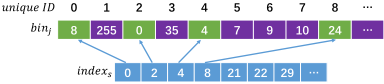
In this section, we show how to speedup our algorithm, specifically the histogram construction, on modern CPUs. With slight abuse of notation, we use n to denote the number of data points in the leaf, and N to denote the size of training set. Each data point has a unique ID, ranging from 1 to N. For each leaf s, an array indexs of length n is maintained to record these ID's for all data points in the leaf. For each feature j, we maintain an array binj of length N. For a data point with unique ID id, binj[id] records which bin the data point falls in the histogram of feature j. With these notations, we summarize the histogram construction process for leaf s and feature j in Algorithm 2. As mentioned in Section 4.1, the multiple terms [hixixTi , gixi] making the histogram construction expensive. Next, we introduce two important techniques to speedup the construction.
Algorithm 2 Histogram Construction for Feature j on Leaf s
- 1: Input: x1, ..., xn, g1, ..., gn, h1, ..., hn, binj, indexs
- 2: Output: histogram histj,s
- 3: for i = 1 to n do
- 4: id = indexs[i]
- 5: bin = binj[id]
- 6: histj,s[bin] += [hixixTi , gixi]
Algorithm 3 SIMD with Reduced Cache Misses
- 1: Input: x1, ..., xn, g1, ..., gn, h1, ..., hn, leafBins,j
- 2: Output: histogram histj,s
- 3: for i = 1 to n do
- 4: bin = leafBins,j[i]
- 5: histj,s[bin] += [hixixTi , gixi] //SIMD add
5.1 SIMD Parallelismwith Reduced Cache Misses
Single Instruction Multiple Data (SIMD) parallelism of modern CPUs supports operations on multiple data items with single instruction. It is obvious that SIMD can be used to speedup line 6 of Algorithm 2, which is a simultaneous addition of multiple items. With SIMD, however, each clock cycle more operands are needed, thus the speedup of SIMD is often bounded by memory bandwidth [Espasa et al., 1998]. In Algorithm 2, when accessing binj , we have to skip the data points not in leaf s (purple blocks in Figure 1). Thus the access to array binj is discontinuous, causing frequent cache misses. To address this problem, we reduce cache misses by rearranging the data structures (a very similar idea is used in LightGBM [Ke et al., 2017] for histogram construction of sparse features).
Suppose leaf s has n data points. For each feature j, we maintain an array leafBins,j of length n to record bin indices of feature j for data points in leaf s. In other words, with the notations in Algorithm 2, for i = 1, ..., n, leafBins,j [i] = binj[indexs[i]]. Since each bin index is stored in a byte, and the access to leafBins,j is continuous, we keep the memory footprint very small and reduces cache misses. Also, with leafBins,j, we can avoid accessing the unique ID array indexs. Histogram construction with leafBins,j using SIMD is summarized in Algorithm 3.
For root node s0, leafBins0,j is exactly binj. When leaf s is split into s1 and s2, leafBins,j is split into leafBins1,j and leafBins2,j accordingly. The split operation has to be done for every feature j. In Section 5.2, we show how to reduce the cost of splitting leafBins,j using Bit Manipulation Instruction Set.
5.2 Using Bit Manipulation Instructions
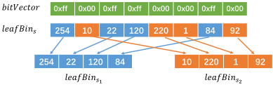
Splitting leafBins,j requires extracting bin indices from leafBins,j and store into leafBins1,j and leafBins2,j. To do this, we need to know for each data point in s, whether it goes to s1 or s2. This information is recorded in a bit vector. Specifically, if s is split with condition xi,k ≤ c, then bitV ector[i]= xi,k ≤ c. Creating bitV ector only requires a single sweep of [x1,k, ..., xn,k]. Then for each feature j, bin indices in leafBins,j are extracted according to bitV ector. BMI is an extension of x86 instructions to speedup bit operations. We use Parallel Bits Extract (PEXT) of BMI to extract the bin indices. PEXT takes two 64-bit registers a and b as operands. For each bit in a whose value is 1, the corresponding bit in b is extracted and stored in the output register. Each bin index is stored in a single byte. Each PEXT instruction can handle 64 bits simultaneously, so we can process 8 bin indices in leafBins,j simultaneously. The workflow of using PEXT is shown in Figure 2. We first broadcast each bit in bitV ector into a byte, thus 1 becomes 0xff and 0 becomes 0x00. Then, with a PEXT instruction, we can extract leafBins1 . Then we negate the bits in bitV ector and extract leafBins2 using another PEXT operation.
6 Experiments
Our experiments aim to answer the following questions 1. How the optimization techniques influence the accuracy and efficiency of boosted PL Trees. 2. How is our algorithm compared with state-of-the-art GBDT packages including LightGBM, XGBoost and CatBoost. We evaluate our algorithm on 10 public datasets. We name our algorithm GBDT-PL. Our code, details of experiment setting and datasets is available at the github page. 1
6.1 Speedup Effects of Optimization Techniques
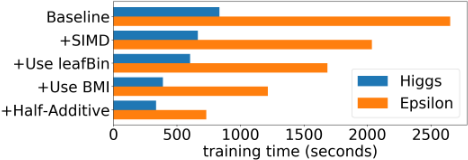
To evaluate the speedup effects of various techniques in Section 4 and 5, we start from a baseline version, and add the optimization techniques incrementally. We record the training time, for 500 iterations using 63 histogram bins, of HIGGS and Epsilon datasets. Figure 3 shows the training time when adding each optimization technique, from top to bottom. The first bar in the top is the baseline version (Algorithm 2 for histogram construction, using fully-corrective fitting). The second bar adds SIMD for histogram construction in Algorithm 2. The third bar uses the leafBin (Algorithm 3). The fourth bar adds Bit Manipulation Instructions (BMI) (Section 5.2). The bottom bar adds the half-additive technique (Section 4.2). Compared with the second bar, the fourth bar with leafBin data structure and BMI gets a speedup of about 1.5 to 2 times. With leafBin we reduce the cache misses when constructing the histograms. With fewer cache misses when getting the bin indices, we can provide operands to the SIMD units in CPUmore efficiently, thus further exploit the computation power. And with BMI, we speedup the split operations of leafBin thus reduces the overhead of maintaining leafBin.
1 https://github.com/GBDT-PL/GBDT-PL.git
| setting | time (s) | AUC | speedup |
|---|---|---|---|
| a. no feat. sel. and half-additive | 8443.75 | 0.859 | ×1.0 |
| b. feat. sel., no half-additive | 574.88 | 0.856 | ×14.7 |
| c. feat. sel., half-additive | 405.07 | 0.854 | ×20.8 |
6.2 Effects of Optimization Techniques on Accuracy
Incremental feature selection restricts the size of linear models, and half-additive fitting results in suboptimal linear model parameters. We evaluate the effects of these two techniques on the accuracy. We test the following 3 settings. a. Disable the half-additive fitting and incremental feature selection. This means all features will be used in linear models of all nodes. b. Enable the incremental feature selection. Set the maximum constraint of regressors to 5. c. Based on b, enable the half-additive fitting. Table 1 shows the results. Here we use 255 histogram bins and 256 leaves. Incremental feature selection and half-additive fitting brings great speedup, with small sacrifice of accuracy. It is expensive to use all features in the linear models for leaves. With incremental feature selection, we restrict the size of linear models to reduce the computational cost. With half-additive fitting, we fits linear models of any size with the cost of 3 regressors. These two techniques are important for the scalability of GBDT-PL.
6.3 Overall Performance
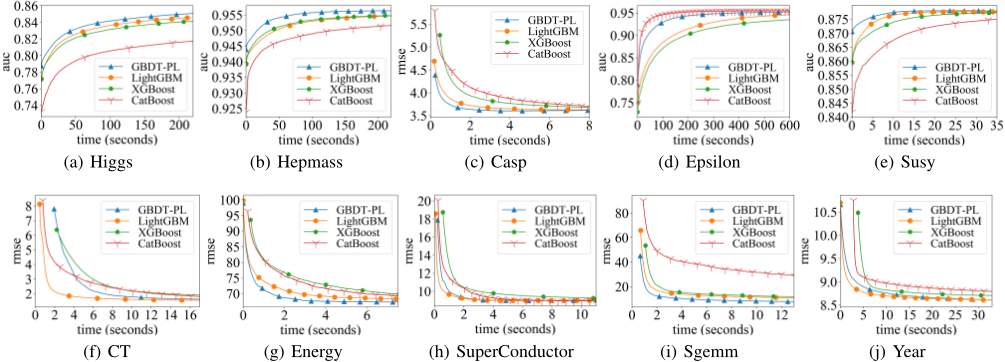
In this section, we compare GBDT-PL with XGBoost, LightGBM and CatBoost, which are state-of-the-art GBDT packages. We compare testing accuracy, convergence rate, and training speed on CPUs.
Accuracy
We evaluate all 10 datasets with the 4 algorithms. For regression datasets Casp, CT, Sgemm, Year, SuperConductor and Energy, we use RMSE as evaluation metric. And for binary classification datasets Higgs, Hepmass, Epsilon and Susy, we use AUC. Different settings of hyperparameters are tried. Key hyperparameters we tuned include: 1. num leaves ∈ {16, 64, 256, 1024}, which controls the size of each tree. For CatBoost with SymmetricTree mode, the tree is grown by level, so max depth ∈ {4, 6, 8, 10} is used instead of num leaves. 2. max bin ∈ {63, 255}, the maximum number of bins in histograms. 3. min sum hessians ∈ {1.0, 100.0}, the sum of hessians of data in each leaf. 4. learning rate ∈ {0.01, 0.05, 0.1}, the weight of each tree. 5. l2 reg ∈ {0.01, 10.0}, l2 regularization for leaf predicted values. We fix the number of regressors used in GBDT-PL to 5 in all runs. Different combinations of these parameters are tried. The maximum number of trees are chosen according to the rule learning rate × num trees = 50 (For CatBoost in SymmetricTree mode we use learning rate×num trees = 200
since it converges slower). For large datasets, only learning rate 0.1 is tried. More details of parameter settings are listed in our github. For XGBoost, LightGBM and CatBoost, result of the best iteration over all settings on test set is recorded. For GBDT-PL, we seperate 20% of training data for validation, and pick the best setting on validation set, then record the corresponding accuracy on test set. Table 2 shows the results. With linear models on leaves, GBDT-PL achieves better accuracy in these dense numerical datasets. It shows greater advantage in regression tasks. The results shows that 5 regressors is enough for most datasets. Adjusting the number of regressors can further improve the results.
Convergence Rate
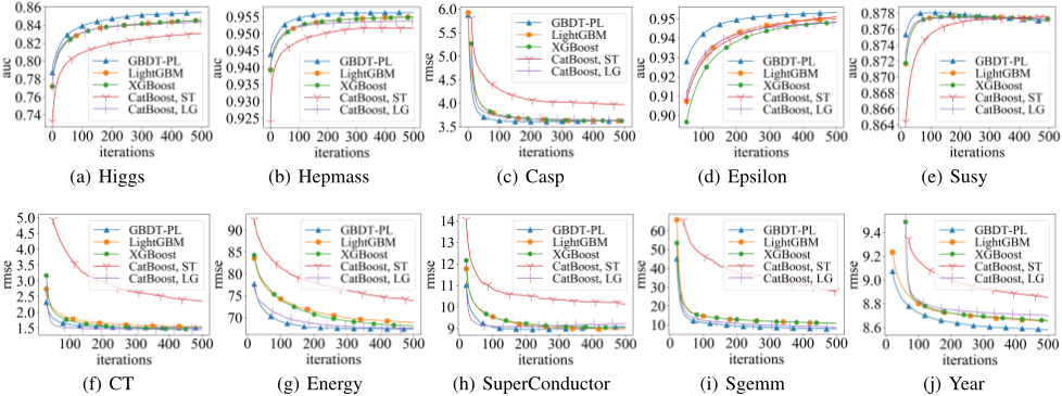
To show that PL Trees speedup the convergence rate of GBDT, we set the maximum number of leaves to 256, and the maximum depth of CatBoost in SymmetricTree mode to 8. We use 63 histogram bins, 500 iterations with learning rate 0.1. We set min sum hessians to 100 and l2 reg to 0.01. Figure 4 plots testing accuracy per iteration. In most datasets, GBDT-PL uses fewer trees to reach a comparable accuracy.
Training Time on CPU
To test the efficiency on CPU, we use the same hyperparameters as previous subsection. (So far only SymmetricTree mode is supported by CatBoost on CPU, so only this mode is tested.) Figure 5 shows testing accuracy by training time. With the same tree size, GBDT-PL achieves better accuarcy with less or comparable training time in most datasets.
7 RelatedWork and Discussions
Boosted PL Trees have several existing implementations. Weka [Hall et al., 2009] and Cubist [Kuhn et al., 2012] use M5/M5' [Quinlan and others, 1992; Wang and Witten, 1997] as base learners. M5/M5' grows the tree in a way similar to piece-wise constant ones, then fits linear models on the nodes after the tree structure has been fixed. By contrast, PL Tree used in our work is designed to greedily reduce the loss at each step of its growing. Whenever a node is split in our PL Tree, we choose the optimal split that will result in the largest reduction in loss, considering the linear models in both child nodes. [Wang and Hastie, 2014] proposes a gradient boosting algorithm using PL Trees as base learners and then apply it to a product demand prediction task. However, the algorithm only uses the first-order gradients. By contrast, GBDT-PL uses second-order gradients, which is important for faster convergence rate of GBDT [Sun et al., 2014]. None of the aforementioned algorithms can handle large scale datasets as SOTA GBDT toolkits. Training scalable single PL Tree has been investigated in [Dobra and Gehrke, 2002]. To the best of our knowledge, GBDT-PL is the first to make boosted PL Trees scalable, by various optimization methods in Section 4 and 5. Currently GBDT-PL only handles numerical features. Both LightGBM and CatBoost handles categorical features. However, GBDT-PL is still feasible for categorical features by first converting them into numerical ones, as is done in CatBoost, which encodes the categorical values with label values. Efficient training of GBDT on GPUs is also a hot topic [Zhang et al., 2018; Wen et al., 2018]. We will add support for GPU in the future.
| Algorithm | Higgs | Hepmass | Casp | Epsilon | Susy | CT | Sgemm | Year | SuperConductor | Energy |
|---|---|---|---|---|---|---|---|---|---|---|
| LightGBM | 0.854025 | 0.95563 | 3.4961 | 0.951422 | 0.878112 | 1.30902 | 4.61431 | 8.38817 | 8.80776 | 64.256 |
| XGBoost | 0.854147 | 0.95567 | 3.4939 | 0.948292 | 0.877825 | 1.34131 | 4.37929 | 8.37935 | 8.91063 | 64.780 |
| CatBoost | 0.851590 | 0.95554 | 3.5183 | 0.957327 | 0.878206 | 1.36937 | 4.41177 | 8.42593 | 8.78452 | 65.761 |
| GBDT-PL | 0.860198 | 0.95652 | 3.4574 | 0.957894 | 0.878287 | 1.23753 | 4.16871 | 8.37233 | 8.79527 | 65.462 |
and accuracy. Comparisons with SOTA baselines show the value of our methods.
Acknowledgements
The research is supported in part by the National Basic Research Program of China Grant 2015CB358700, the National Natural Science Foundation of China Grant 61822203, 61772297, 61632016, 61761146003, and a grant from Microsoft Research Asia.
8 Conclusions
In this paper, we propose efficient GBDT with PL Trees. We first extend GBDT with second-order approximation for PL Trees. Then incremental feature selection and half-additive fitting are proposed to efficiently fit the linear models in tree nodes. Finally, we show how to exploit SIMD parallelism and reduce cache misses by rearranging the data structures with Bit Manipulation Instructions. The proposed optimization techniques are tested to show their effects on efficiency
@inproceedings{ijcai2019p476,
  title     = {Gradient Boosting with Piece-Wise Linear Regression Trees},
  author    = {Shi, Yu and Li, Jian and Li, Zhize},
  booktitle = {Proceedings of the Twenty-Eighth International Joint Conference on
               Artificial Intelligence, {IJCAI-19}},
  publisher = {International Joint Conferences on Artificial Intelligence Organization},
  editor    = {Sarit Kraus},
  pages     = {3432--3438},
  year      = {2019},
  month     = {8},
  note      = {Main track},
  doi       = {10.24963/ijcai.2019/476},
  url       = {https://doi.org/10.24963/ijcai.2019/476},
}
TY - CPAPER TI - Gradient Boosting with Piece-Wise Linear Regression Trees AU - Shi, Yu AU - Li, Jian AU - Li, Zhize T2 - Proceedings of the Twenty-Eighth International Joint Conference on Artificial Intelligence, IJCAI-19 PB - International Joint Conferences on Artificial Intelligence Organization PY - 2019 SP - 3432 EP - 3438 DO - 10.24963/ijcai.2019/476 UR - https://doi.org/10.24963/ijcai.2019/476 ER -Copied
Machine-readable versions of this paper, for tools and AI agents:





