
Influence of State-Variable Constraints on Partially Observable Monte Carlo Planning
Proceedings of the Twenty-Eighth International Joint Conference on Artificial Intelligence. Main track. Pages 5540-5546.
https://doi.org/10.24963/ijcai.2019/769
Keywords
- Planning and Scheduling: Robot Planning
- Planning and Scheduling: POMDPs
Abstract
Online planning methods for partially observable Markov decision processes (POMDPs) have recently gained much interest. In this paper, we propose the introduction of prior knowledge in the form of (probabilistic) relationships among discrete state-variables, for online planning based on the well-known POMCP algorithm. In particular, we propose the use of hard constraint networks and probabilistic Markov random fields to formalize state-variable constraints and we extend the POMCP algorithm to take advantage of these constraints. Results on a case study based on Rocksample show that the usage of this knowledge provides significant improvements to the performance of the algorithm. The extent of this improvement depends on the amount of knowledge encoded in the constraints and reaches the 50% of the average discounted return in the most favorable cases that we analyzed.
- [Amato and Oliehoek, 2015] Christopher Amato and Frans A. Oliehoek. Scalable Planning and Learning for Multiagent POMDPs. In Proc. AAAI'15, pages 1995-2002. AAAI Press, 2015.
- [Bishop, 2006] Christopher M. Bishop. Pattern Recognition and Machine Learning. Springer-Verlag New York, 2006.
- [Boutilier et al., 1999] Craig Boutilier, Thomas Dean, and Steve Hanks. Decision-theoretic Planning: Structural As- sumptions and Computational Leverage. JAIR, 11(1):1- 94, 1999.
- [Browne et al., 2012] Cameron Browne, Edward Powley, Daniel Whitehouse, Simon Lucas, Peter Cowling, Philipp Rohlfshagen, Stephen Tavener, Diego Perez, Spyridon Samothrakis, and Simon Colton. A Survey of Monte Carlo Tree Search Methods. IEEE Trans. Comp. Intell. AI Games, 4(1):1-43, 2012.
- [Castellini et al., 2018] Alberto Castellini, Giovanni Bel- trame, Manuele Bicego, Jason Blum, Matteo Denitto, and Alessandro Farinelli. Unsupervised activity recognition for autonomous water drones. In Proc. SAC 2018, pages 840-842. ACM, 2018.
- [Dechter, 2003] Rina Dechter. Constraint Processing. Mor- gan Kaufmann Pub. Inc., San Francisco, CA, USA, 2003.
- [Duranti, 2015] Pierluigi Duranti. CatOne, Multitask Un- manned Surface Vessel for Hydro-Geological and Environ- ment Surveys, pages 647-652. Springer, 2015.
- [Farinelli et al., 2012] Alessandro Farinelli, Daniele Nardi, Roberta Pigliacampo, Mirco Rossi, and Giuseppe Settem- bre. Cooperative situation assessment in a maritime sce- nario. Int. J. Intelligent Systems, 27(5):477-501, 2012.
- [Ferri et al., 2015] Gabriele Ferri, Alessandro Manzi, Francesco Fornai, Francesco Ciuchi, and Cecilia Laschi. The HydroNet ASV, a Small-Sized Autonomous Cata- maran for Real-Time Monitoring of Water Quality: From Design to Missions at Sea. IEEE J. Oceanic Engineering, 40(3):710-726, 2015.
- [Griffith and Pradalier, 2015] Shane Griffith and Cedric Pradalier. A Spatially and Temporally Scalable Approach for Long-Term Lakeshore Monitoring. In Field and Service Robotics, volume 113 of Springer Tracts in Advanced Robotics, pages 3-16. Springer, 2015.
- [Hamza and Ayanian, 2017] Ameer Hamza and Nora Aya- nian. Forecasting Battery State of Charge for Robot Mis- sions. In Proc. SAC 2017, pages 249-255. ACM, 2017.
- [Hauskrecht, 2000] Milos Hauskrecht. Value-Function Ap- proximations for Partially Observable Markov Decision Processes. JAIR, 13:33-94, 2000.
- [J. D. Williams, 2005] S. Young J. D. Williams, P. Poupart. Factored partially observable Markov decision processes for dialogue management. In Proc. 4th Workshop on Knowledge and Reasoning in Practical Dialog Systems, IJCAI 2005, pages 76-82, 2005.
- [Kaelbling et al., 1998] Laslie Kaelbling, Michael Littman, and Anthony Cassandra. Planning and Acting in Partially Observable Stochastic Domains. Artificial Intelligence, 101(1-2):99-134, 1998.
- [Kocsis and Szepesvári, 2006] Levente Kocsis and Csaba Szepesvári. Bandit Based Monte-Carlo Planning. In Proc. ECML'06, pages 282-293, Berlin, Heidelberg, 2006. Springer-Verlag.
- [Lee et al., 2018] Jongmin Lee, Geon-Hyeong Kim, Pascal Poupart, and Kee-Eung Kim. Monte-Carlo Tree Search for Constrained POMDPs. In NIPS'18, pages 1-17, 2018.
- [LeSage and Longoria, 2013] J. LeSage and R. Longoria. Characterization of Load Uncertainty in Unstructured Ter- rains and Applications to Battery Remaining Run-time Prediction. J. Field Robotics, 30(3):472-487, 2013.
- [McAllester and Singh, 1999] David McAllester and Satin- der Singh. Approximate Planning for Factored POMDPs using Belief State Simplification. In Proc. UAI '99, pages 409-416, 1999.
- [Müller et al., 2012] Felix Müller, Christian Späth, Thomas Geier, and Susanne Biundo. Exploiting Expert Knowledge in Factored POMDPs. In Proc. ECAI'12, pages 606-611. IOS Press, 2012.
- [Murphy, 2012] Kevin Murphy. Machine Learning: A Prob- abilistic Perspective. The MIT Press, 2012.
- [Papadimitriou and Tsitsiklis, 1987] Christos Papadimitriou and John Tsitsiklis. The Complexity of Markov Decision Processes. Math. Oper. Res., 12(3):441-450, August 1987.
- [Ross et al., 2008] Stephane Ross, Joelle Pineau, Sebastien Paquet, and Brahim Chaib-draa. Online Planning Algo- rithms for POMDPs. JAIR, 32:663-704, 2008.
- [Russell and Norvig, 2003] Stuart Russell and Peter Norvig. Artificial Intelligence: A Modern Approach. Pearson Edu- cation, 2 edition, 2003.
- [Sadrpour et al., 2012] Amir Sadrpour, Jionghua Jin, and Galip Ulsoy. Mission energy prediction for unmanned ground vehicles. In ICRA, pages 2229-2234, 2012.
- [Silver and Veness, 2010] David Silver and Joel Veness. Monte-Carlo Planning in Large POMDPs. In NIPS'10, pages 2164-2172, 2010.
- [Smith and Simmons, 2004] Trey Smith and Reid Simmons. Heuristic Search Value Iteration for POMDPs. In Proc. UAI '04, pages 520-527, 2004.
- [Sutton and Barto, 2018] Richard Sutton and Andrew Barto. Reinforcement Learning, An introduction. MIT Press, Cambridge, MA, USA, 2nd edition, 2018.
- [Thrun et al., 2005] Sebastian Thrun, Wolfram Burgard, and Dieter Fox. Probabilistic Robotics (Intelligent Robotics and Autonomous Agents). The MIT Press, 2005.
- [Thrun, 2000] Sebastian Thrun. Monte Carlo POMDPs. In NIPS'00, pages 1064-1070. MIT Press, 2000.
References were extracted automatically from the PDF and may contain errors.
Full text extracted automatically from the PDF; figures, tables and equations may differ. The PDF is the version of record.
1 Introduction
Planning in large uncertain environments is a key task for autonomous and intelligent agents [Boutilier et al., 1999]. Several approaches and modeling frameworks were developed to deal with this problem in research fields as artificial intelligence [Russell and Norvig, 2003] and robotics [Thrun et al., 2005]. Partially Observable Markov Decision Processes (POMDPs) [Kaelbling et al., 1998] provide a standard framework for modeling uncertainty in dynamical environment. They combine the strengths of Hidden Markov Models [Bishop, 2006] and Markov Decision Processes [Russell and Norvig, 2003], by capturing dynamics that depend on both unobserved states and effects of sequential decisions.
Computing optimal policies [Sutton and Barto, 2018] for POMDPs is a complex task. Since solving POMDPs exactly is computationally intractable [Papadimitriou and Tsitsiklis, 1987], a lot of effort was put on approximate [Hauskrecht, 2000] and online [Ross et al., 2008] algorithms, and in recent years impressive progress was made in this direction. Many improvements were derived from the use of Monte Carlo Tree Search (MCTS) [Browne et al., 2012], that have enabled the solution of problems with very large state spaces. This search strategy can find optimal solutions by taking random samples in the decision space and building a search tree according to the results obtained from the simulation of these samples. The first POMDP solvers based on Monte Carlo search dates back to 2000 [Thrun, 2000], but the pioneer algorithm for more recent improvements is arguably Partially Observable Monte Carlo Planning (POMCP) [Silver and Veness, 2010], which combines a Monte Carlo update of the agent's belief state with an MCTS-based policy.
In this paper, we aim at solving specific planning problems in which the hidden state is described by n discrete statevariables, and also some prior knowledge is available about the relationships between state-variables values. There exist several problems having this structure. A synthetic one is the well-known Rocksample [Smith and Simmons, 2004], in which state-variables represent (unknown) rock values, and some plausible prior knowledge can be provided by relationships between rock values (e.g., rocks with similar color or shape could have higher probability to have equal value). A real-world problem having the same structure is that of intelligent battery management for aquatic drones [Farinelli et al., 2012; Duranti, 2015; Ferri et al., 2015; Griffith and Pradalier, 2015; Castellini et al., 2018]. Since battery consumption is heavily influenced by environmental factors, such as, flowing current and wind, state-variables can be used in this context to represent the difficulty level of path segments (in terms of energy requirements), and state-variables relationships to represent the similarity between segment difficulties, which depends on the similarity between environmental features. Equivalent problems can be found also in unmanned aerial and ground vehicles [Sadrpour et al., 2012; LeSage and Longoria, 2013; Hamza and Ayanian, 2017].
We propose two methods for representing state-variable relationships, namely, constraint networks (CNs) [Dechter, 2003] and Markov random fields (MRFs) [Bishop, 2006; Murphy, 2012]. The first enables the definition of hard constraints, the second the use of probabilistic constraints. Then, we present a novel extension of the POMCP algorithm that takes advantage of the prior knowledge introduced by these constraints. Finally, we compare the performance (in terms of average discounted return) of the standard POMCP algorithm with that of its extended versions, and quantify the impact of different amounts and types (hard/probabilistic) of constraints on this performance. Results show that POMCPs take advantage of prior knowledge about state-variable relationships, in terms of both improved average discounted return and speed to accumulate the reward.
The contribution of this work is three-fold:
- we formalize the problem of Partially Observable Monte Carlo Planning with state-variable relationships;
- we extend the POMCP algorithm with CNs and MRFs to cope with constraints between state-variables;
- we systematically analyze the performance of the extended POMCP depending on different levels of prior knowledge introduced by state-variable constraints.
The rest of the paper is organized as follows. Section 2 presents related work. Section 3 formalizes our extension to POMCPs. In Section 4 results on Rocksample are described. Section 5 draws conclusions and directions for future work.
2 RelatedWork
Some recent work concerns the improvement of planning performance in specific application contexts where assumptions can be made regarding the structure of the problem. An example is [Amato and Oliehoek, 2015], in which the multiagent structure of a problem is used to decompose the value function into a set of overlapping factors that enable scalability and performance improvements in POMCP. Also [Lee et al., 2018] recently presented a scalable extension of POMCP for dealing with cost constraints while maximizing rewards. However, this work solves a different problem: we use constraints on the state space to refine the belief space and increase performance (in terms of less actions or shorter execution time), while [Lee et al., 2018] proposes cost-constraints to solve problems with multiple objectives. Other related work concerns factored POMDPs and their applications [M¨uller et al., 2012; J. D. Williams, 2005; McAllester and Singh, 1999]. Our perspective is however substantially different, since we do not propose a specific factored POMDP framework but the extension of an online planning method to incorporate prior knowledge on the domain.
3 Methods
We formalize the problem, describe CNs and MRFs for representing state-variable relationships, and introduce extended POMCPs that use this knowledge for policy generation.
3.1 ProblemFormalization
A POMDP [Kaelbling et al., 1998] is a tuple (S,A,O, T,Z,R, γ), where S is a finite set of states, A is a finite set of actions, Z is a finite set of observations, T: S × A → Π(S) is the state-transition model, O: S × A → Π(Z) is the observation model, R: S × A → R is the reward function and γ ∈ [0, 1) is a discount factor. The goal of an agent operating a POMDP, is to maximize its expected total discounted reward (also called discounted return) E[∑∞t=0 γ tR(st, at)], by choosing the best action at in each state st at time t; γ is used to reduce the weight of distant rewards and ensure the (infinite) sum's convergence.
In this context, we define a planning problem in which the (hidden) state s is fully described by n discrete statevariables, called X1, . . . ,Xn. Hence, a specific configuration (x1, x2, . . . , xn) of all state-variables fully describes the hidden state, where xi ∈ D and D = {d1, . . . , dk} is the domain of all state-variables. For instance, in the well-known Rocksample problem, state-variables X1, . . . , Xn are the (unknown) values of rocks and D = {0, 1}, where 1 represents a valuable rock and 0 a valueless rock. A possible hidden state could be s = (0, 1, 1, 1, 0), i.e., the first and last rocks are valueless, and the second, third and fourth rocks are valuable. In the intelligent battery management problem for aquatic drones, mentioned in the introduction, state-variables could represent difficulties of path segments, with D containing values for low, medium and high segment difficulty.
Given a planning problem of such form, the POMCP algorithm [Silver and Veness, 2010] can be used to compute a policy π which approximates the optimal one. The policy π is computed online using Monte-Carlo Tree Search [Browne et al., 2012]: for any observed history ht = {a1, o1, . . . , at, ot} (i.e., a sequence of actions and observations), MCTS assigns to a tree node a value V π (ht) ∈ R, namely the expected discounted cumulative return from history ht when following policy π. That is, V π (ht) = Eπ[∑∞k=t γ k-t rk],
Let us assume now to have some probabilistic prior knowledge about the relationships between state-variables. For instance, we could know that P(X1 = X5) = 0.9, namely, the probability the value of rock 1 is equal to the value of rock 5 is 90%. Intuitively, this knowledge can be used to constrain the belief state and to improve the performance (e.g., average discounted return) of the policy computed online by POMCP. In other words, if we call π′ the policy generated by using the knowledge about state-variable relationships and π the policy generated without considering that knowledge, then the value of π′ should be at least as good as the value of π. 1 Hence, for each history ht, we have that V π′ (ht) = V π (ht) + Gπ′ R (ht), where Gπ′ R (ht) ≥ 0 is a gain in the return quantity derived from following π′ instead of π.
The goal of this paper is to experimentally characterize the aforementioned gain as a function of the prior knowledge provided on state-variable relationships in the specific context of the POMCP algorithm. To this end, we first describe how knowledge about state-variable relationships can be mathematically formalized, and then explain how to modify the POMCP algorithm to exploit this new knowledge.
3.2 Representation of State-Variable Relationships
State-variable relationships are the additional input to the POMCP algorithm that we use to improve planning performance. This knowledge can be represented in several ways. Here we propose two such representation methods, namely CNs and MRFs. The first allows the definition of hard constraints, the second is a generalization to probabilistic constraints. The two representations are then used in Section 4 to characterize two kinds of influence between state-variable constraints and planning performance.
1 This is easily proved to be actually a certainty-unless the prior information is flawed.
Constraint Networks
A constraint network [Dechter, 2003] R is a triple (X, D, C) consisting of a set of variables X = {X1, . . . , Xn}, with respective domains D = {D1, . . . , Dn} which list the possible values for each variable Di = {di1, . . . , viki }, and a set of constraints C = {C1, . . . , Cu}. Each constraint Ci is a relation Qi defined on a subset of variables Yi ⊆ X. The relation denotes the variables' simultaneous legal values assignments. Yi is called the scope of Qi. If Yi = {Xi1 , . . . ,Xir }, then Qi is a subset of the Cartesian product Di1 , . . . ,Dir . Hence, a constraint is also a pair Ci = 〈Yi, Qi〉.
In our context, constraint network variables X are represented by state-variables (we used the same notation for both concepts), the domain of all variables coincide and are represented by the sets Di = {d1, . . . , dk} of statevariable values (e.g., {0, 1} for Rocksample's rock values). Each constraint Ci = 〈Yi,Qi〉, where Yi = {Xi1 ,Xi2 } and Qi = {(dj, dj), j = 1, . . . , k}, represents the fact that two state variables Xi1 and Xi2 have the same values. As an example, in Rocksample the constraint Ci = 〈{X1,X5}, {(0, 0), (1, 1)}〉 represents the equality between rocks 1 and 5, which is equivalent to the notation P(X1 = X5) = 1 used above.
Pairwise MRFs
Dependencies between pairs of state variables can be represented via undirected graphs, where nodes represent statevariables and edges represent probabilistic relationships between state-variables. The theory of MRFs [Bishop, 2006; Murphy, 2012] can be used to factorize the joint probability of segment difficulties as a product of potential functions over the maximal cliques of the graph, according to the Hammersley-Clifford theorem. The joint probability is p(x|θ) = 1 Z(θ) ∏q∈Q ψq(xq|θq) where x is a vector of statevariables (e.g., (0, 1, 1, 0, 0) in the Rocksample problem), θ is a parameterization of the MRF, Q is the set of (maximal) cliques of the graph, ψq(xq|θq) is a potential function for clique q and Z(θ) = ∑x ∏q∈Q ψq(xq|θq) is a normalization factor called partition function.
We use pairwise MRF, a particular type of MRF where the parametrization is restricted to the edges of the graph rather than to the maximal cliques, hence set Q corresponds to the set of relations in constraint networks. We conveniently express potentials as exponentials, so that ψq(xq|θq) = exp(-E(xq|θq)) where E(xq) is called energy function, and the exponential representation is a Boltzmann distribution. In this way, the product of potentials can be computed by adding the energies of all pairwise relationships.
Since our state-variables are discrete, we represent the potentials as matrices of (non-negative) numbers representing the relative "compatibility" between different assignments of state-variables. For instance, given a pair of state-variables (Xi,Xj) | i, j ∈ {1, . . . , n} in Rocksample, their potential could be, ψXiXj (0, 0) = 0.45 which indicates a probability of 0.45 to have value 0 in both rocks Xi and Xj, or ψXiXj (0, 1) = 0.05, which indicates a probability of 0.05 to have value 0 in rock Xi and 1 in rock Xj .
3.3 Standard POMCP Algorithm
The standard POMCP algorithm [Silver and Veness, 2010] does not consider prior knowledge about state-variable relationships. Here we provide a description of the main elements of this algorithm, and in the next section we introduce an extension that uses this knowledge.
Particle initialization. POMCP starts with a MCTS containing only the root node representing the empty history h (no action performed and no observation observed). The belief state is represented by a particle filter which is initialized with K particles. The particles in the root node are initialized by a procedure that selects random hidden states (e.g., rock value configurations in Rocksample) from a uniform distribution over all possible hidden states. This procedure is called Standard Particle Initialization (SPI) in the following.
Simulations and node statistics update. At each step POMCP performs nSim simulations from the current history h to generate (online) a policy for that step. A particle, representing a state s of the system, is randomly chosen from the particle filter of node h which represents the belief state of the agent. At each simulation step 2 , an action a is selected using the Upper Confidence Bound for Trees (UCT) method [Kocsis and Szepesv´ari, 2006] when the current history is inside the tree, and a uniform policy when the current history is outside the tree. A black-box simulator G(s, a) is used to perform a simulation step, it returns a simulated observation and a simulated reward. When all simulation steps are performed, the total reward of the simulation is used to update node statistics about the average return of all simulations passing through h.
Action selection in the real environment. Real actions (performed in the real environment) are selected, once again, by the UTC strategy, which uses the statistics of the root node.
Belief update. When an action a is applied to the real environment a real observation o is obtained, the belief is updated according to the evidence collected by moving particles to the new history node hao, the tree root is moved to node hao and the rest of the tree is pruned. Notice that both the constraint probabilities and the evidence collected step by step influence the belief state over time.
Particle reinvigoration. If a lack of particles is experienced, then new particles are generated by computing local transformations on current particles. These transformations concern the modification of the value of a single statevariable. Specific local transformations may be defined depending on the problem of interest.
3.4 Extending the POMCP Algorithm
To enable the introduction of state-variable relationships two kinds of change to the POMCP algorithm can be implemented, namely, (i) new particle initialization strategies can be used to initialize the particle filter with states that satisfy state-variable constraints, (ii) new particle reinvigoration strategies can be used to generate new states that satisfy the constraints in the vicinity of current states.
2 The term step is used to identify steps in the real environment; the term simulation step to identify steps in the simulation phase.
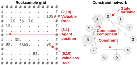
Particle initialization for constraint networks. The particles in the belief state of the empty history node are initialized by considering the (hard) constraints in the constraint network. We first compute the connected components of the constraint network. Each component identifies a set of statevariables that must have equal values (e.g., nodes 0-2-3 in Figure 1 must have same values since they are in the same connected component). For each particle (i.e., vector of statevariables) to be initialized, we randomly select a value d ∈ D for each connected component and set all the variables in the connected component to this value. This procedure, which can be simply extended to non-equality constraints, is called Constraint Network Initialization (CNI) in the following.
Particle initialization for MRF. This procedure aims at initializing particles in the belief state according to the probabilistic constraints defined by a MRF. We first generate a large number N of uniformly random particles (we used N = 10000 in our experiments). Each random particle is a specific configuration of state-variable values. Then, we compute the joint probability of each particle by the formulae in Section 3.2. Finally, we select K particles by considering their probability distribution, namely, each particle has a probability to be selected which is proportional to its joint probability. This basic sampling procedure, called MRF Initialization (MRFI) in what follows, ensures that the distribution of the initial belief satisfies the probabilistic constraints defined by the MRF. More advanced sampling methods, such as rejection or importance sampling [Thrun et al., 2005; Bishop, 2006], may be considered for specific applications.
Particle reinvigoration. We performed particle reinvigoration using the same sampling strategies used for particle initialization, namely CNI or MRFI depending on the type of constraint representation. We noticed, however, that reinvigoration positively affects (on average) planning performance only when the size of the state space is much larger than the number of particles used by POMCP.
3.5 Characterization of Performance Gain
As mentioned above, the question we want to answer in this work is: how does the average cumulative discounted return of the POMCP policy changes with respect to changes in state-variable relationship constraints? As an extreme example, if a constraint network is defined which forces all the state-variables of a Rocksample problem with 11 rocks to have the same values, then only two possible configurations of the rock values can be considered, namely, all valuable rocks or all valueless rocks. Of course the search in this small space makes the policy synthesis problem much simpler then in the standard case and, consequently, the average discounted return is expected to grow. Similar analysis could be performed considering the policy value, instead of the discounted return, as an "expected" performance measure. Next section presents a systematic experimental analysis of these dependencies in the general case of probabilistic constraints.
4 Experimental Evaluation
We present and discuss results achieved by extended POMCPs on Rocksample with different levels of prior knowledge.
4.1 The Rocksample Case Study
We tested our approach on Rocksample(11,11) [Smith and Simmons, 2004], in which 11 rocks are randomly arranged on a grid with 11 rows and 11 columns. Figure 1 shows an instance of the problem having a particular placement of the rocks in the grid (known by the agent), a specific configuration of rock values (hidden state-variables) and an agent position (observable state-variable). Notation (i, j) is used to identify the cell in row i and column j (from the top-left corner of the grid). For instance, cell (8,10) contains symbol 9X which represents the valueless rock 0, while cell (2,10) contains symbol 10$ which represents the valuable rock 10. Hash marks represent grid bounds and the asterisk in cell (6,1) shows the current agent position. In our tests, rock positions are fixed and known by the agent, while rock values, which are unknown by the agent, are randomly chosen at each run from a Bernoulli distribution with probability p = 0.5, hence they are uniformly distributed in {0, 1}.
At each step, the agent can perform one action among moving (North, South, East or West), sampling a rock (i.e., getting the rock) and checking a rock. In the last case, the probability to observe the correct value of one rock is inversely proportional to the distance between the agent and the rock. The reward is 0 in case of moving and checking, 10 if a valuable rock is sampled and -10 if a valueless rock is sampled. If the agent hits the rightmost border it gets a reward of 10 and the run ends. The policy should suggest actions that maximize the discounted reward over runs of 100 steps. In order to get statistically sound results, we averaged the discounted return over 50 runs, and provided mean performance and standard errors. Tests with different number of simulations nSim were performed. In particular, we repeated each of the 50 runs for nSim from 23 = 8 to 214 = 16384, with steps of the power of 2. Test parameters are displayed in Table 1 and corresponding results shown in Figure 2.
4.2 Planning Strategies
The original C++ code of the POMCP algorithm provided in [Silver and Veness, 2010] was used to perform tests in the standard case (STD). The same code was modified in two ways to obtain an oracle planner (ORC) and a constrained state-variable planner (CSV). The oracle was made by forcing the particle filter of POMCP to contain only the true state of the system. In the following we call this initialization strategy oracle particles initialization (OPI). Using the ORC planner the agent's belief is always correct and all the simulations are performed considering the real configuration of rock values, which is a key advantage to obtain correct policies and high returns. The CSV planner, instead, employs particle initialization and reinvigoration described in Section 3.4, that guarantee an exploration of the state space considering probabilistic constraints on state-variables.
4.3 Experiment Design and Results
We performed two kinds of experiments on the CSV planner, one to evaluate the influence of the number of state-variable constraints on planning performance, and one to evaluate the influence of uncertainty over state-variable constraints on planning performance.
Influence of the Number of State-Variable Constraints
In the first set of experiments we used hard constraints, namely constraints that must be satisfied by state-variable configurations in order to be considered valid, and we analyzed the variation of average discounted return corresponding to the variation of the number of constraints. In particular, we set equality constraints between pairs of state-variables that actually have the same values in the real state.
We observed that the performance of the CSV planner does not depend on the number of constraints, but it depends on the number of connected components in the constraints network, since this number actually constrains the state space. We tested the performance of the CSV planner with constraint networks having 8, 5, and 2 connected components, and compared their performance to that of the STD and ORC planners. In Table 1, these tests are referenced as E1 for the STD planner; E2 for the ORC planner; and E3, E4, E5 for the CSV planner with 8, 5, and 2 components, respectively. Notice that the STD planner corresponds to the CSV planner with 11 connected components (i.e., no edge in the constraint network), since there are 11 state-variables in Rocksample(11,11).
For each experiment, we performed 50 runs for each specific number of simulations (as described in Section 4.1). Figure 2(a) shows the average discounted return (across all 50 runs) for the different number of simulations. In the bottom lies the blue line for the STD planner which has the lowest performance, with a maximum average discounted return of about 14 when 16384 simulations are performed. Then the CSV planners with 8, 5 and 2 connected components, called CSV 8 CC, CSV 5 CC and CSV 2 CC, respectively, have increasing performance, with a maximum average discounted return of about 21 (+50% with respect to the STD planner) by CSV 2 CC when 16384 simulations are performed. Finally, the ORC planner has the best performance with an average discounted return of almost 25 with 16384 simulations.
We computed also the average cumulative discounted reward and the average cumulative policy value of each of the five planners when 16384 simulations are performed. They are two measures of the speed and capability of the planner to accumulate reward over time. The first considers the sum of the reward actually obtained from the real environment, while the second considers the sum of the potential reward expected step by step by the agent according to the policy which it updates online according to the POMCP strategy. Figure 2(b) shows that the order of performance is kept, with ORC (red line) reaching the maximum cumulative average reward with the highest speed, followed by CSV 2 CC (dark green line), then by CSV 5 CC and CSV 8 CC (respectively, green and light green line) which have similar final values but different speeds (i.e., CSV 5 CC is faster than CSV 8 CC, as expected); finally, STD has lower final performance in terms of both final value and speed. The curves of cumulative policy values are not displayed for space reasons but they show a similar behavior. Time performance of different approaches depend on the number of simulations performed at each step but no correlation is observed between the number of connected components in the constraint network and the average time needed to complete each run.
Influence of Uncertainty in State-Variable Constraints
In the second set of experiments we analyzed the influence of uncertainty about state-variable constraints on planning performance. We used probabilistic constraint networks based on pairwise MRF and set network edges in the same way we did in the first set of experiments (i.e., using only equality constraints between some pairs of state-variables actually having same values in the real state). However, instead of setting the constraint probabilities to 1 (hard constraints) we set them to decreasing values 0.9, 0.7, 0.5 and 0.2, in different experiments called respectively E6, E7, E8 and E9 (see Table 1). The number of connected components in the network was always set to 2. As an example, in experiment E6 we set all edge probabilities (i.e., potentials), to 0.9. This means that for every pair of connected state-variables, the probability that they have same value is 0.9, therefore they could be different. Notice that the planner with edge potentials equal to 0.5 (i.e., experiment E8) corresponds to the STD planner, since probability 0.5 corresponds to no prior knowledge. On the other hand, edge potentials equal to 0.2 (i.e., experiment E9) correspond to deceptive constraints, since they put small equality probability to pairs actually having equal state-variables.
Comparisons between different aspects of the performance of planners ORC, CSV 2 CC (MRF 1.0), CSV 2 CC (MRF 0.9), CSV 2 CC (MRF 0.7), CSV 2 CC (MRF 0.5) and CSV 2 CC (MRF 0.2) are displayed in the right-hand side column of Figure 2. In particular, Figure 2(c) shows decreasing average discounted return of the six planners. As expected, ORC has the best performance since it uses only the true state, then comes CSV 2 CC (MRF 1.0) which explores only a 4-dimensional space of states, and subsequently come the planners with edge potentials 0.9, 0.7 and 0.5, in which the soft constraints potentially enable to explore the complete state space, but in practice the exploration is probabilistically focused on states close to the true real state. We notice that the trend of average discounted return of CSV 2 CC (MRF 0.5) in Figure 2(c) is similar to that of STD in Figure 2(a), as expected, with a value of about 14 for 16384 simulations in both cases. Of interest is CSV 2 CC (MRF 0.2), whose performance is worse than the standard because the knowledge provided is deceptive (it explores states far from the true one).
| Exp name | Planning algorithm | Constraint representation | Particle init./reinv. | # connected components | Edge potentials |
|---|---|---|---|---|---|
| E1 | STD | No | SPI | 11 | - |
| E2 | ORC | No | OPI | - | - |
| E3 | CSV 8 CC | CN | CNI | 8 | 1.0 |
| E4 | CSV 5 CC | CN | CNI | 5 | 1.0 |
| E5 | CSV 2 CC | CN | CNI | 2 | 1.0 |
| E6 | CSV 2 CC (MRF 0.9) | MRF | MRFI | 2 | 0.9 |
| E7 | CSV 2 CC (MRF 0.7) | MRF | MRFI | 2 | 0.7 |
| E8 | CSV 2 CC (MRF 0.5) | MRF | MRFI | 2 | 0.5 |
| E9 | CSV 2CC (MRF 0.2) | MRF | MRFI | 2 | 0.2 |
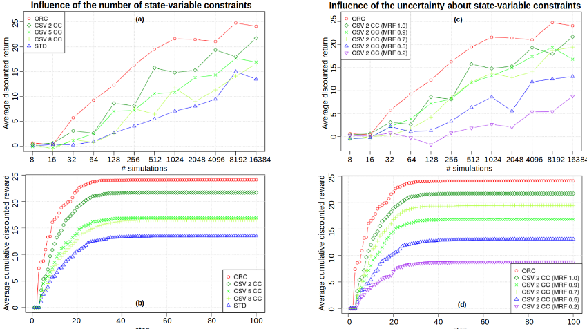
The analysis of average cumulative discounted rewards across run steps in the case of 16384 simulations (see Figure 2(d)) shows that the order of performance is similar to that displayed in Figure 2(c), namely the smaller the edge potentials the smaller the average cumulative reward and the speed of accumulation of the reward itself. However, in this specific case the performance of CSV 2 CC (MRF 0.7) was higher than that of CSV 2 CC (MRF 0.9) for nSim = 16384 (see Figure 2(c)), and this inversion is kept also in cumulative discounted reward. Also in this case the average time per run has no correspondence with the amount of knowledge (i.e., number of edge potentials) injected in the constraint network.
5 Conclusions and FutureWork
We analyzed the influence of probabilistic constraints among state-variables in POMCP planning according to two dimensions of analysis, namely, i) the relationship between the number of connected components and planning performance, and ii) the relationship between constraint uncertainty and planning performance. Results shown that POMCP can take advantage of prior knowledge about state-variable relationships, in terms of both improved average discounted return and speed to accumulate the reward. Future developments concern the application of the proposed approach to a real case study of battery management in autonomous robots, and the theoretical characterization of bounds on the gain in discounted return Finally, we intend to investigate the scaling potential of our methodology.
Acknowledgments
This work is funded by the European Union's Horizon 2020 research and innovation program (grant 689341), and by the MIUR program "Dipartimenti di Eccellenza 2018-2022.
@inproceedings{ijcai2019p769,
  title     = {Influence of State-Variable Constraints on Partially Observable Monte Carlo Planning},
  author    = {Castellini, Alberto and Chalkiadakis, Georgios and Farinelli, Alessandro},
  booktitle = {Proceedings of the Twenty-Eighth International Joint Conference on
               Artificial Intelligence, {IJCAI-19}},
  publisher = {International Joint Conferences on Artificial Intelligence Organization},
  editor    = {Sarit Kraus},
  pages     = {5540--5546},
  year      = {2019},
  month     = {8},
  note      = {Main track},
  doi       = {10.24963/ijcai.2019/769},
  url       = {https://doi.org/10.24963/ijcai.2019/769},
}
TY - CPAPER TI - Influence of State-Variable Constraints on Partially Observable Monte Carlo Planning AU - Castellini, Alberto AU - Chalkiadakis, Georgios AU - Farinelli, Alessandro T2 - Proceedings of the Twenty-Eighth International Joint Conference on Artificial Intelligence, IJCAI-19 PB - International Joint Conferences on Artificial Intelligence Organization PY - 2019 SP - 5540 EP - 5546 DO - 10.24963/ijcai.2019/769 UR - https://doi.org/10.24963/ijcai.2019/769 ER -Copied
Machine-readable versions of this paper, for tools and AI agents:





