Evaluating Approval-Based Multiwinner Voting in Terms of Robustness to Noise

1 Introduction

Voting has received much attention by the AI community recently, mostly due to its suitability for simple and effective decision making. One popular line of research, that originates from Arrow [1951], has aimed to characterize voting rules in terms of the social choice axioms they satisfy. Another approach views voting rules as estimators. It assumes that there is an objectively correct choice, a ground truth, and votes are noisy estimates of it. Then, the main criterion for evaluating a voting rule is whether it can determine the ground truth as outcome when applied to noisy votes.

A typical scenario in studies that follow the second approach employs a hypothetical noise model that uses the ground truth as input and produces random votes. Then, a voting rule is applied on profiles of such random votes and is considered effective if it acts as a maximum likelihood estimator [Conitzer and Sandholm, 2005; Young, 1988] or if it has low sample complexity [Caragiannis et al., 2016]. As such evaluations are heavily dependent on the specifics of the noise model, relaxed effectiveness requirements, such as the accuracy in the limit, sought in broad classes of noise models [Caragiannis et al., 2016] can be more informative.

We restrict our attention to approval voting, where ballots are simply sets of alternatives that are approved by the voters [Laslier and Sanver, 2010]. Furthermore, we consider multiwinner voting rules [Faliszewski et al., 2017], which determine committees of alternatives as outcomes [Kilgour, 2010; Aziz et al., 2017]. In particular, we focus on approvalbased counting choice rules (or, simply, ABCC rules), which were defined recently by Lackner and Skowron [2018]. A famous rule in this category is known as multiwinner approval voting (AV). Each alternative gets a point every time it appears in an approval vote and the outcome consists of a fixed number of alternatives with the highest scores.

We consider noise models that are particularly tailored for approval votes and committees. These models use a committee as ground truth and produce random sets of alternatives as votes. We construct broad classes of noise models that share a particular structure, parameterized by distance metrics defined over sets of alternatives. In this way, we adapt to approval-based multiwinner voting the approach of Caragiannis et al. [2016] for voting rules over rankings.

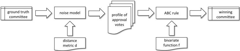
Figure 1 illustrates our evaluation framework. The noise model is depicted at the left. It takes as input the ground truth committee and its probability distribution over approval votes which is consistent to a distance metric d. Repeated executions of the noise model produce a profile of random approval votes. The ABCC rule (defined using a bivariate function f; see Section 2) is then applied on this profile and returns one or more winning committees. Our requirement for the ABCC rule is to be accurate in the limit (informally, on profiles with infinitely many votes, it must return the ground truth as the unique winning committee), not only for a single noise model, but for all models that belong to a sufficiently broad class. The breadth of this class quantifies the robustness of the ABCC rule to noise.

The details of our framework are presented in Section 2. Our results indicate that it indeed allows for a classification of ABCC rules in terms of their robustness to noise. In particular, we identify (in Section 3) the modal committee rule (MC) as the ultimately robust ABCC rule: MC is robust against all kinds of reasonable noise. AV follows in terms of robustness and seems to outperform other known ABCC rules (see Section 4). In contrast, the well-known approval ChamberlinCourant (CC) rule is the least robust. On the other hand, all ABCC rules are robust if we restrict noise sufficiently (see Section 5). We conclude with a discussion on open problems in Section 6.

Further related work. Approval-based multiwinner voting rules have been studied in terms of their computational complexity [Aziz et al., 2015; Skowron et al., 2016], axiomatic properties [S´anchez-Fern´andez et al., 2017; Lackner and Skowron, 2018; Aziz et al., 2017], as well as their applications [Brill et al., 2017]. In particular, axiomatic work has focused on two different principles that govern multiwinner rules: diversity and individual excellence. Lackner and Skowron [2019] attempt a quantification of how close an approval-based multiwinner voting rule is to these two principles. We remark that the primary focus of the current paper is on individual excellence.

The robustness of approval voting has been previously evaluated against noise models, using either the MLE [Procaccia and Shah, 2015] or the sample complexity [Caragiannis and Micha, 2017] approach. These papers assume a ranking of the alternatives as ground truth, generate approval votes that consist of the top alternatives in rankings produced according to the noise model of Mallows [1957], and assess how well approval voting recovers the ground truth ranking. We believe that our framework is fairer to approval votes, as recovering an underlying ranking when voters have very limited power to rank is very demanding. The robustness of (non-approval) multiwinner voting against noise has been studied by Procaccia et al. [2012]. Different notions of robustness in multiwinner voting are considered by Gawron and Faliszewski [2019] and Bredereck et al. [2017].

2 Preliminaries

Throughout the paper, we denote by A the set of alternatives. We use m = |A| and denote the committee size by k. The term committee refers to a set of exactly k alternatives.

Approval-based multiwinner voting. An approval vote is simply a subset of the alternatives (of any size). An approvalbased multiwinner voting rule takes as input a profile of approval votes and returns one or more winning committees.

We particularly consider voting rules that belong to the class of approval-based counting choice rules (or, simply, ABCC rules), introduced by Lackner and Skowron [2018]. Such a rule is defined by a bivariate function f, with f(x, y) indicating a non-negative score a committee gets from an approval vote containing y alternatives, x of which are common with the committee. f is non-decreasing in its first argument.

Formally, f is defined on the set Xm,k, which consists of all pairs (x, y) of possible values of |U ∩ S| and |S|, given that U is k-sized and S can be any subset of the m alternatives of A. I.e., Xm,k is the set

The score of a committee is simply the total score it gets from all approval votes in a profile. Winning committees are those that have maximum score. We extensively use "the ABCC rule f" to refer to the ABCC rule that uses the bivariate function f. We denote the score that an ABCC rule f assigns to the committee U given a profile Π = (Si)i∈[n] of n votes by scf (U, Π) = ∑ni=1 f(|U ∩ Si|, |S|). With some abuse of notation, we use scf(U, Si) to refer to the score U gets from vote Si. Hence, scf (U, Π) = ∑ni=1 scf (U, Si).

Well-known ABCC rules include:

• Multiwinner approval voting (AV), which uses the function fAV(x, y) = x.
• Approval Chamberlin-Courant (CC), which uses the function fCC(x, y) = min{1, x}. The rule falls within a more general context considered by Chamberlin and Courant [1983].
• Proportional approval voting (PAV), which uses the function fPAV(x, y) = ∑xi=1 1/i.

These rules belong to the class of rules that originate from the work of Thiele [1895]. A Thiele rule uses a vector 〈w1, w2, ..., wk〉 of non-negative weights to define f(x, y) = ∑xi=1 wj . Other known Thiele rules include the p-Geometric rule [Skowron et al., 2016] and Sainte Lagu¨e approval voting [Lackner and Skowron, 2019].

A well-known non-Thiele rule is the satisfaction approval voting (SAV) rule that uses fSAV(x, y) = x/y for y > 0 and f(x, y) = 0 otherwise [Brams and Kilgour, 2014]. Let us also introduce the modal committee (MC) rule 1 which returns the committee (or committees) that has maximum number of appearances as approval votes in the profile. MC is also nonThiele; it uses f(k, k) = 1 and f(x, y) = 0 otherwise.

Noise models. We employ noise models to generate approval votes, assuming that the ground truth is a committee. Denoting the ground truth by U ⊆ A, a noise model M produces random approval votes according to a particular distribution that defines the probability PrM[S|U] to generate the set S ⊆ A when the ground truth is U.

1 We remark that MC is similar in spirit to the modal ranking rule considered by Caragiannis et al. [2014].

Let us give the following noise model Mp as an example. Mp uses a parameter p ∈ (1/2, 1]. Given a ground truth committee U, Mp generates a random set S ⊆ A by selecting each alternative of U with probability p and each alternative in A \ U with probability 1 - p. Intuitively, the probability that a set will be generated depends on its "distance" from the ground truth: the higher this distance, the smaller this probability. To make this formal, we will need the set difference 2 distance metric d∆ : 2A → R≥0 defined as d∆(X, Y ) = |X \ Y | + |Y \ X|.

So, the probability PrMp [S|U] is decreasing in d∆(U, S). We will consider general noise models M with PrM[S|U] depending on d(U, S), where d is a distance metric defined over subsets of A.

Definition 1. Let d be a distance metric over sets of alternatives. A noise model M is called d-monotonic if for any two sets S1, S2 ⊆ A, it holds PrM[S1|U] > PrM[S2|U] if and only if d(U, S1) < d(U, S2).

Besides the set difference metric used by Mp, other wellknown distance metrics 3 (see Deza and Deza [2016]) are:

• the normalized set difference or Jaccard metric dJ, defined as dJ (X, Y ) = d∆(X,Y ) |X∪Y | ,
• the maximum difference or Zelinka metric dZ, defined as dZ(X, Y ) = max{|X \ Y |, |Y \ X|}, and
• the normalized maximum difference or Bunke-Shearer metric dBS, defined as dBS(X, Y ) = dZ(X,Y ) max{|X|,|Y |} .

Evaluating ABCC rules against noise models. We aim to evaluate the effectiveness of ABCC rules when applied to random profiles generated by large classes of noise models. To this end, we use accuracy in the limit as a measure.

Definition 2 (accuracy in the limit). An ABCC rule f is called accurate in the limit for a noise model M if for every ε > 0 there exists nε such that, for every profile with at least nε approval votes produced by Mwith ground truth U, f returns U as the unique winning committee with probability at least 1 - ε.

Then, ABCC rules are evaluated in terms of robustness using the next definition.

Definition 3 (robustness). Let d be a distancemetric over sets of alternatives. An ABCC rule f is monotone robust against d (or d-monotone robust) if it is accurate in the limit for all d-monotonic noise models.

2 Viewing sets as strings, the distance metric d∆ is equivalent to the Hamming distance; see [Deza and Deza, 2016].

3 Notice that d(X, Y ) for the four specific distance metrics defined here depends only on |X \ Y |, |Y \ X|, |X|, and |Y |. In a sense, these distance metrics are alternative-independent. Our results apply to the most general definition of distance, where d(X, Y ) can also depend on the contents of X \ Y , Y \ X, X, and Y .

3 MC is a Uniquely Robust ABCCRule

We begin our technical exposition by identifying the unique ABCC rule that is monotone robust against all distance metrics. Our proofs, in the current and subsequent sections, make extensive use of the following lemma. The notation S ∼ M(U) indicates that the random set S is drawn from the noise model M with ground truth U .

Lemma 2. LetMbe a noise model. An ABCC rule f is

1. accurate in the limit for M if ES∼M(U)[scf(U, S) - scf(V, S)] > 0 for every two different sets of alternatives U, V ⊆ A with |U| = |V | = k.
2. not accurate in the limit forMif ES∼M(U)[scf(U, S)- scf(V, S)] < 0 for some pair of sets of alternatives U, V ⊆ A with |U| = |V | = k.

Due to lack of space, the proof of Lemma 2 is omitted. We are ready to present our first application of Lemma 2.

Theorem 3. MC is the only ABCC rule that is monotone robust against any distance metric.

Proof. LetMbe a noise model that is d-monotonic for some distance metric d. Let U, V ⊆ A be any two different k-sized sets of alternatives. By the definition of MC, we have

By Lemma 2a, we obtain that MC is d-monotone robust.

We will now show that MC is the only ABCC rule f that has this property. Let f be an ABCC rule that is different than MC. This means that there exist integers x∗ and y∗ with (x∗ - 1, y∗ ), (x∗ , y∗ ) ∈ Xm,k, (x∗ , y∗ ) ̸= (k, k), and f(x∗ , y∗ ) > f(x∗ - 1, y∗ ). We will construct a distance metric d and a d-monotonic noise model for which f is not accurate in the limit.

Rename the alternatives of A as a1, a2, ..., am and let U = {a1, a2, ..., ak}, V = {a2, ..., ak+1}, and W = {ak-x∗+2, ..., ay∗+k-x+1}. Notice that, by the definition of Xm,k, (x∗ - 1, y∗ ) ∈ Xm,k implies that 1 +max{y∗ + k - m, 0} ≤ x∗ and, equivalently, y∗ + k - x∗ + 1 ≤ m; hence, the set W is well-defined. Clearly, x∗ ≥ 1; so sets V and W share at least one alternative.

We define a distance metric between subsets of A that has d(X, Y ) = 0 if X = Y , d(X, Y ) ∈ {1, 2}, otherwise, and in particular d(U, V ) = d(U,W) = 1 and d(U, S) = 2 for every S different than U, V , or W.

We are ready to define the d-monotonic noise model M. For simplicity, we use p0 = PrM[U|U], p1 = PrM[V |U] = PrM[W|U], and p2 = PrM[S|U] for every other set S ⊆ A different than U, V , or W. For δ > 0 (to be specified shortly), we set p0 = 1/3, p1 = 1/3- δ, and p2 = 2δ 2m-3 .

We now compute the quantity ES∼M(U)[scf(U, S) - scf(V, S)]; observe that scf(U,U) = scf(V, V ) = f(k, k), scf (U, V ) = scf (V, U ) = f (k - 1, k), scf (U, W ) = f (x∗ - 1, y∗ ), and f(V,W) = f(x∗ , y∗ ). We obtain

Observe that the RHS of (1) is increasing in δ and approaches - 13 (f(x∗ , y∗ )-f(x∗ -1, y∗ )) < 0 as δ approaches 0. Hence, for a sufficiently small positive δ, we have

By Lemma 2b, f is not accurate in the limit forM.

4 ACharacterization for AV

In this section, we identify the class of distance metrics against which AV is monotone robust. We will need some additional notation that will be useful in several proofs.

For a distance metric d and a set of alternatives U, let span(d,U) be the number of different non-zero values the quantity d(U, ·) can take. We denote these different distance values by δ1(d,U), δ2(d,U), ..., δspan(d,U)(d,U). We also use δ0(d,U) = 0. For t = 0, 1, ..., span(d,U) and alternatives a, b ∈ A, we denote by N ta|b (d,U) the class of sets of alternatives S that contain alternative a but not alternative b and satisfy d(U, S) ≤ δt(d, U).

Definition 4 (majority-concentricity). A distance metric d is called majority-concentric 4 if for every k-sized set of alternatives U, it holds N ta|b (d,U) ≥ N t b|a (d,U) for every alternatives a ∈ U and b ̸∈ U and t = 0, 1, ..., span(d, U).

We are ready to prove our characterization for AV.

Theorem 4. AV is d-monotone robust if and only if the distance metric d is majority-concentric.

Proof. Let M be a d-monotonic noise model for a majority concentric distance metric d. Let U and V be two different sets with k alternatives each. By Lemma 2a, in order to show that AV is accurate in the limit for M (and, consequently, d-monotone robust), it suffices to show that ES∼M(U)[scAV(U, S) - scAV(V, S)] > 0.

We will need some additional notation. For t = 0, 1, ..., span(d, U), we denote by ¯N t (d, U)) the class of sets of alternatives S that satisfy d(U, S) = δt(d,U). For alternatives a, b ∈ A, we denote ¯N ta (d,U)) the subclass of

4 Majority-concentricity is similar in spirit with a property of distance metrics over rankings with the same name in [Caragiannis et al., 2016].

¯N t (d, U) consisting of sets of alternatives that include a and by ¯N ta|b (d,U) the subclass of ¯N ta (d,U) consisting of sets do not contain alternative b.

To simplify notation, we set s = span(d,U). Also, we drop (d,U) (e.g., we use N ta|b instead of N ta|b (d,U)) from notation since it is clear from context. We have

Now, observe that the probability PrM[S|U] is the same for all sets S ∈ ¯N t . In the following, we use pt = PrM[S|U] for all S ∈ ¯N t , for t = 0, 1, ..., s. Hence, (2) becomes

Similarly, we have

and, by linearity of expectation,

Let µ be a bijection that maps each alternative of V \ U to a distinct alternative of U \ V . Then, (3) becomes

The third equality follows since ¯N 0 a|µ(a) = N 0 a|µ(a) , ¯N 0 µ(a)|a = N 0 µ(a)|a , and ¯N ta|µ(a) = N ta|µ(a) \ N t-1 a|µ(a) and ¯N tµ(a)|a = N tµ(a)|a \N t-1 µ(a)|a for t = 1, ..., s. The first inequality follows since d is majority concentric and since pt > pt+1 and, thus, all differences in (4) are non-negative. The last inequality follows after observing that since |N 0 a|µ(a) | = 1 and |N 0 µ(a)|a | = 0 for a ∈ U \ V and since p0 > p1. This completes the "if" part of the proof.

Let us now consider a non-majority concentric distance metric d that satisfies N t∗ a|b (d,U) < N t∗ b|a (d,U) for the ksized set of alternatives U, some alternatives a ∈ U and b ̸∈ U, and some t∗ ∈ {1, 2, ..., span(d,U)}. We show the "only if" part of the theorem by constructing a noise model M that satisfies ES∼M(U)[scAV(U, S) - scAV(V, S)]<0 for V = U \ {a} ∪ {b}.

Again, we use pt = PrM[S|U] for every set of alternatives S ∈ ¯N t (d,U), s = span(d,U), and drop (d,U) from notation. We define the model probabilities so that τ = p0 > p1 > ... > pt∗ = τ - ϵ and 2ϵ = pt∗+1 > ... > ps = ϵ. Notice that such a noise model exists for any arbitrarily small ϵ > 0. Since there are 2m sets of alternatives and τ is the probability that M returns the ground truth ranking, it must be τ > 1/2m. We now apply equality (4). Observe that, since V = U \ {a} ∪ {b}, µ(a) = b. We obtain

Now, observe that for t ̸= t∗ , it holds |N ta|b | - |N t b|a | ≤ 2m (the total number of sets of alternatives) and pt - pt+1 ≤ ϵ. Also, |N t∗ a|b | - |N t∗ b|a | ≤ -1 and pt∗ -pt∗+1 = τ -3ϵ. Setting specifically ϵ = 1 s8m , we obtain that

which is negative for m ≥ 2 since s ≥ 1. The proof of the "only if" part of the theorem now follows by Lemma 2b.

It is tempting to conjecture that AV and MC are the only ABCC rules that are monotone robust against all majority concentric distance metrics. However, this is not true as the next example, which uses a different ABCC rule, shows.

Example 1. Let A = {a, b, c} and k = 2. Consider the majority concentric distance metric d and the ABCC rule f with f (1, 1) = 1, f (2, 2) = 2, and f (x, y) = 0 otherwise. We will show that f is d-monotone robust against any majority concentric distance metric d. Without loss of generality, let us assume that U = {a, b} and V = {a, c}. Observe that the quantity scf(U, S) - scf(V, S) is equal to 0 when S = ∅, {a}, {b, c}, {a, b, c}, 1 when S = {b}, -1 when S = {c}, 2 when S = {a, b}, and -2 when S = {a, c}. Hence, for the d-monotonic noise model M, we have ES∼M(U)[scf (U, S)- scf(V, S)] = 2pab - 2pac + pb - pc, where pab, pac, pb, and pc are abbreviations for the probabilities PrM[S|U] for S = {a, b}, {a, c}, {b}, and {c}, respectively.

In order to have N t b|c ≥ N t c|b for t = 0, 1, ..., span(d,U) as the definition of majority concentricity requires, it must be either pab > pb, pc ≥ pac or pab > pb, pac ≥ pc. In the first case, we have ES∼M(U)[scf (U, S) - scf (V, S)] = (pab - pac) + (pab - pc) + (pb - pac) > 0. In the second case, we have ES∼M(U)[scf (U, S) - scf (V, S)] = 2(pab - pac)+(pb -pc) > 0. Accuracy in the limit of the ABCC rule f for the noise model M then follows by Lemma 2a.

5 Robustness of Other ABCCRules

Our results for ABCC rules different than MC and AV involve two classes of distance metrics. We define the first one here.

Definition 5 (natural distance). A distance metric d is called natural if for every three sets U, V , and S with |U| = |V | such that |U ∩S| > |V ∩S|, it holds that d(U, S) ≤ d(V, S).

The next observation follows easily by the definitions.

Claim 5. Any natural distance metric is majority-concentric. The opposite is not true as the next example illustrates.

Example 2. Let A = {a, b, c} and consider the distance metric with d(X, Y ) = 0 for every pair of sets with X = Y , d(X, Y ) = 1 if X ∩ Y = ∅ and X ∪ Y = A, and d(X, Y ) = 2, otherwise. It can be easily seen that the distance is majority-concentric; it suffices to observe that, within distance 1 from any set, each alternative appears in exactly one set. To see that is not natural, consider U = {a, b}, V = {a, c} and S = {b}. We have |U ∩ S| > |V ∩ S| but d(U, S) = 2 > 1 = d(V, S).

Lemma 7 below identifies the class of ABCC rules that are monotone robust against all natural distance metrics. The condition uses an appropriately defined bijection on sets of alternatives.

Definition 6. Given two different sets U and V with |U| = |V |, a (U, V )-bijection µ : 2A → 2A is defined as µ(S) = {µ′ (a) : a ∈ S}, where µ′ : A → A is such that µ′ (a) = a for every alternative a ∈ U ∩ V or a ̸∈ U ∪ V , µ′ (a) is a distinct alternative in V \ U for a ∈ U \ V , and µ′ (a) is a distinct alternative in U \ V for a ∈ V \ U.

It is easy to see that a (U, V )-bijection µ has the following properties.

Claim 6. Let U, V ⊆ A with |U| = |V | and let µ be a (U, V )- bijection. For every S ⊆ A, it holds |S| = |µ(S)|, |U ∩ S| = |V ∩ µ(S)|, and |U ∩ µ(S)| = |V ∩ S|.

Lemma 7. An ABCC rule is d-monotone robust against a natural distance metric d if for every two different sets of alternatives U, V ⊆ A with |U| = |V | = k there exists a (U, V )-bijection µ on sets of alternatives and a set S ⊆ A with scf (U, S) > scf (V, S) and d(U, S) < d(U, µ(S)).

Proof. Let U and V be two different sets with k alternatives each. Let S+, S-, and S0 be the classes of sets of alternatives S with |U ∩S| > |V ∩S|, |U ∩S| < |V ∩S|, and |U ∩S| = |V ∩ S|, respectively. Using this notation, we have

We will now transform the third sum in the RHS of (5) to one running over the sets of S+ like the first sum.

Let µ be a (U, V )-bijection on sets of alternatives; by Claim 6, µ maps every set of S- to a set of S+ and viceversa. Hence, instead of enumerating sets of S-, we could enumerate sets of S+ and apply the bijection µ on them. The third sum in the RHS of (5) then becomes

The second equality follows since, by Claim 6, scf (U, µ(S)) = f (|U ∩µ(S)|, |µ(S)|) = scf (|V ∩S|, |S|) = scf (V, S) and, similarly, scf (V, µ(S)) = scf (U, S).

Now observe that scf(U, S) = scf(V, S) when S ∈ S0. Hence, the second sum in the RHS of (5) is equal to 0. By combining (5) and (6), we get

Now observe that the RHS of (7) is always non-negative. This is due to the fact that S ∈ S+ which implies that scf (U, S) = f(|U ∩ S|, |S|) ≥ f(|V ∩ S|, |S|) = scf (V, S) since f is non-decreasing in its first argument and d(U, S) ≤ d(U, µ(S)) (and, consequently, PrM[S|U] ≥ PrM[µ(S)|U]) since d is natural and, by Claim 6, |U ∩ S| > |V ∩ S| = |U ∩ µ(S)|. The RHS of (7) is strictly positive if there exists a set S ∈ S+ that further satisfies d(U, S) < d(U, µ(S)) (and, consequently, PrM[S|U] > PrM[µ(S)|U]) and scf (U, S) > scf (V, S). The lemma then follows by Lemma 2a.

We now present two applications of Lemma 7.

Theorem 8. An ABCC rule f is monotone robust against any natural distance metric if and only if f(k, k) > f(k - 1, k).

Notice that most popular ABCC rules from Section 2 satisfy the condition of Theorem 8. CC is an exception. The omitted proof of Theorem 8 implies that CC is not monotone robust for the natural distance metric d defined as d(X, Y ) = 0 if X = Y and d(X, Y ) = 1, otherwise.

Our second application of Lemma 7 involves all non-trivial ABCC rules and an important subclass of natural distances.

Definition 7 (similarity distance). A natural distance metric d is a similarity distance metric if for every three sets U, V , and S with |U| = |V | such that |U ∩ S| > |V ∩ S|, it holds that d(U, S) < d(V, S).

Theorem 9. Any non-trivial ABCC rule is monotone robust against any similarity distance metric.

Proof. We apply Lemma 7 assuming a non-trivial ABCC rule f and a similarity distance metric d. Non-triviality of f implies that for every two different sets U and V with k alternatives each, there is a set S such that scf(U, S) > scf(V, S). This yields |U ∩ S| > |V ∩ S| = |U ∩ µ(S)|, where µ is any (U, V )-bijection (see Claim 6), and implies that d(U, S) < d(U, µ(S)) since d is a similarity distance.

We can easily show that the four distance metrics set difference, Jaccard, Zelinka, and Bunke-Shearer that we defined in Section 2 are all similarity distance metrics. Using this observation and Theorem 9, we obtain the next statement.

Corollary 10. Any non-trivial ABCC rule is monotone robust against the set difference, Jaccard, Zelinka, and BunkeShearer distance metrics.

6 Epilogue

We believe that our approach complements nicely the axiomatic and quantitative analysis of approval-based multiwinner voting. The current paper leaves many interesting open problems. Besides identifying ABCC rules that are at least as robust as AV, applying our framework to non-ABCC rules deserves investigation. Beyond assessing the effects of noise in the limit, studying the sample complexity of approval-based multiwinner voting is important. This will require the design of concrete noise models like the Mp model that we presented in Section 2. In particular, models that simulate user behaviour in crowdsourcing platforms will be useful for evaluating approval-based voting in such environments. Even though the Mp model is very simple, we expect that implementation issues will emerge for more elaborate noise models. Similar issues in the implementation of the Mallows [1957] ranking model have triggered much non-trivial work; see, e.g., [Doignon et al., 2004].

Acknowledgments

This research is co-financed by Greece and the European Union (European Social Fund) through the Operational Programme "Human Resources Development, Education and Lifelong Learning 2014-2020" (project MIS 5047146).