
Discovering Latent Class Labels for Multi-Label Learning
Proceedings of the Twenty-Ninth International Joint Conference on Artificial Intelligence. Main track. Pages 3058-3064.
https://doi.org/10.24963/ijcai.2020/423
Keywords
- Machine Learning: Multi-instance;Multi-label;Multi-view learning
- Machine Learning: Classification
- Data Mining: Classification, Semi-Supervised Learning
Abstract
Existing multi-label learning (MLL) approaches mainly assume all the labels are observed and construct classification models with a fixed set of target labels (known labels). However, in some real applications, multiple latent labels may exist outside this set and hide in the data, especially for large-scale data sets.
Discovering and exploring the latent labels hidden in the data may not only
find interesting knowledge but also help us to build a more robust learning model.
In this paper, a novel approach named DLCL (i.e., Discovering Latent Class Labels for MLL) is proposed which can not only discover the latent labels in the training data but also predict new instances with the latent and known labels simultaneously.
Extensive experiments show a competitive performance of DLCL against other
state-of-the-art MLL approaches.
- [Beck and Teboulle, 2009] A. Beck and M. Teboulle. A fast iterative shrinkage-thresholding algorithm for linear in- verse problems. SIAM J. Imaging Sci., 2(1):183-202, 2009.
- [Boutell et al., 2004] M. R. Boutell, J.-B. Luo, X.-P. Shen, and C. M. Brown. Learning multi-label scene classifica- tion. Pattern Recognit., 37(9):1757-1771, 2004.
- [Chen et al., 2019] C. Chen, H. Wang, W. Liu, X. Zhao, T. Hu, and G. Chen. Two-stage label embedding via neu- ral factorization machine for multi-label classification. In AAAI, pages 3304-3311, 2019.
- [Demšar, 2006] J. Demšar. Statistical comparisons of clas- sifiers over multiple data sets. JMLR, 7:1-30, 2006.
- [Gibaja and Ventura, 2015] E. Gibaja and S. Ventura. A tutorial on multilabel learning. ACM Comput. Surv., 47(3):52:1-52:38, 2015.
- [Hu and Chen, 2019] M.-L. Hu and S.-C. Chen. One-pass incomplete multi-view clustering. In AAAI, pages 3838- 3845, 2019.
- [Hua and Qi, 2008] X.-S. Hua and G.-J. Qi. Online multi- label active annotation: Towards large-scale content-based video search. In ACM MM, pages 141-150, 2008.
- [Huang et al., 2016] J. Huang, G. Li, Q. Huang, and X. Wu. Learning label-specific features and class-dependent labels for multi-label classification. IEEE Trans. Knowl. Data Eng., 28(12):3309-3323, 2016.
- [Huang et al., 2018] J. Huang, G. Li, Q. Huang, and X. Wu. Joint feature selection and classification for multilabel learning. IEEE Trans. Cybern., 48(3):876 -889, 2018.
- [Huang et al., 2019] J. Huang, F. Qin, X. Zheng, Z. Cheng, Z. Yuan, W. Zhang, and Q. Huang. Improving multi-label classification with missing labels by learning label-specific features. Inf. Sci., 492:124-146, 2019.
- [Jain et al., 2019] H. Jain, V. Balasubramanian, B. Chunduri, and M. Varma. Slice: Scalable linear extreme classifiers trained on 100 million labels for related searches. In WS- DM, pages 528-536, 2019.
- [Jia and Zhang, 2019] B.-B. Jia and M.-L. Zhang. Multi- dimensional classification via knn feature augmentation. In AAAI, pages 3975-3982, 2019.
- [Kuzborskij et al., 2013] I. Kuzborskij, F. Orabona, and B. Caputo. From n to n+1: Multiclass transfer incremental learning. In CVPR, pages 3358-3365, 2013.
- [Nguyen et al., 2016] V. Nguyen, T. D. Nguyen, T. Le, S. Venkatesh, and D. Phung. One-pass logistic regression for label-drift and large-scale classification on distributed systems. In ICDM, pages 1113-1118, 2016.
- [Pham et al., 2015] A. Pham, R. Raich, X. Fern, and J. P. Ar- riaga. Multi-instance multi-label learning in the presence of novel class instances. In ICML, pages 2427-2435, 2015.
- [Tan et al., 2018] Q. Tan, G. Yu, C. Domeniconi, J. Wang, and Z. Zhang. Incomplete multi-view weak-label learning. In IJCAI, 2018. IJCAI
- [Wang et al., 2019] H. Wang, W. Liu, Y. Zhao, C. Zhang, T. Hu, and G. Chen. Discriminative and correlative partial multi-label learning. In IJCAI, pages 3691-3697, 2019. IJCAI
- [Wei et al., 2019] T. Wei, W.-W. Tu, and Y.-F. Li. Learning for tail label data: A label-specific feature approach. In IJCAI, pages 3842-3848, 2019. IJCAI
- [Wu et al., 2019] X. Wu, Q. Chen, Y. Hu, D. Wang, X. Chang, X. Wang, and M.-L. Zhang. Multi-view multi- label learning with view-specific information extraction. In IJCAI, pages 3884-3890, 2019.
- [Xing et al., 2018] Y. Xing, G. Yu, C. Domeniconi, J. Wang, and Z. Zhang. Multi-label co-training. In IJCAI, 2018.
- [Xioufis et al., 2011] E. S. Xioufis, M. Spiliopoulou, G. T- soumakas, and I. Vlahavas. Dealing with concept drift and class imbalance in multi-label stream classification. In IJ- CAI, pages 1583-1588, 2011. IJCAI
- [Xu et al., 2019] N. Xu, J. Lv, and X. Geng. Partial label learning via label enhancement. In AAAI, pages 3838- 3845, 2019.
- [Yang et al., 2016] H. Yang, J. T. Zhou, and J. Cai. Improv- ing multi-label learning with missing labels by structured semantic correlations. In ECCV, pages 835-851, 2016.
- [Yu et al., 2014] H. Yu, P. Jain, P. Kar, and I. S. Dhillon. Large-scale multi-label learning with missing labels. In ICML, pages 593-601, 2014.
- [Zhang and Wu, 2015] M.-L. Zhang and L. Wu. Lift: Multi- label learning with label-specific features. IEEE Trans. Pattern Anal. Mach. Intell., 37(1):107-120, 2015.
- [Zhang and Zhou, 2007] M.-L. Zhang and Z.-H. Zhou. Ml- knn: A lazy learning approach to multi-label learning. Pat- tern Recognit., 40(7):2038-2048, 2007.
- [Zhang and Zhou, 2014] M.-L. Zhang and Z.-H. Zhou. A review on multi-label learning algorithms. IEEE Trans. Knowl. Data Eng., 26(8):1819-1837, 2014.
- [Zhang et al., 2018] Y. Zhang, R. Henao, Z. Gan, Y. Li, and L. Carin. Multi-label learning from medical plain text with convolutional residual models. In MLHC, pages 280-294, 2018.
- [Zhang et al., 2020] Y. Zhang, Y. Wang, X.-Y. Liu, S. Mi, and M.-L. Zhang. Large-scale multi-label classification using unknown streaming images. Pattern Recognit., page 107100, 2020.
- [Zhu et al., 2017a] Y. Zhu, K.-M. Ting, and Z.-H. Zhou. Dis- cover multiple novel labels in multi-instance multi-label learning. In AAAI, pages 2977-2983, 2017.
- [Zhu et al., 2017b] Y. Zhu, K.-M. Ting, and Z.-H. Zhou. New class adaption via instance generation in one-pass class incremental learning. In ICDM, pages 1207-1212, 2017.
- [Zhu et al., 2018] Y. Zhu, K.-M. Ting, and Z.-H. Zhou. Multi-label learning with emerging new labels. IEEE Trans. Knowl. Data Eng., 30(10):1901-1914, 2018.
References were extracted automatically from the PDF and may contain errors.
Full text extracted automatically from the PDF; figures, tables and equations may differ. The PDF is the version of record.
1 Introduction
MLL [Zhang and Zhou, 2014; Gibaja and Ventura, 2015] deals with data examples with multiple class labels simultaneously. Many well-known approaches have been proposed to solve different problems of MLL, such as partial MLL [Wang et al., 2019; Xu et al., 2019], extreme MLL [Wei et al., 2019; Jain et al., 2019; Chen et al., 2019], missing labels [Yu et al., 2014; Yang et al., 2016; Tan et al., 2018], and multi-view MLL [Xing et al., 2018; Wu et al., 2019]. It is noted that existing approaches mainly assume that all the class labels are observed in advance. However, in some applications, some latent labels might be completely unobserved and hidden in the data, and below is a summary of two possible reasons:
- Labeling Cost. In the big data era, it is difficult to provide a complete label set for a data, especially a largescale data with an extreme number of labels. Labelling efforts usually focus on the given set of target labels, while labels outside this set will not be considered.
- Limitation of knowledge. For example, in medical diagnosis, possible diseases will be predicted according to
∗ corresponding authors
the patient's symptoms by the model constructed on the history data [Zhang et al., 2018]. However, complicated diseases may definitely exist but have not been discovered due to the limitation of human's knowledge.
Discovering and exploring the class labels hidden in the data may not only find interesting knowledge but also improve the performance on known labels [Pham et al., 2015; Zhu et al., 2017a]. Therefore, it is important to construct a robust model for MLL which can not only discover the latent labels but also could predict new data examples with both the known and latent labels simultaneously.
Approaches have been proposed to solve data classification with an unfixed label set, such as online learning for single-label learning (SLL) [Kuzborskij et al., 2013; Nguyen et al., 2016; Zhu et al., 2017b] and MLL [Hua and Qi, 2008; Xioufis et al., 2011; Zhu et al., 2018; Zhang et al., 2020], However, in the settings of online learning, novel labels are only induced by new instances, and they will not be discovered if they are hidden in the existing training data. MIMLNC [Pham et al., 2015] and DMNL [Zhu et al., 2017a] are two highly related studies on discovering new label(s) for multiinstance multi-label learning (MIMLL). MIMLNC is a probabilistic model to identify novel instances for MIMLL, but it assumes that all novel instances belong to a single new label. DMNL tries to discover multiple novel labels for MIMLL. It assumes that there are k novel labels, and the problem is formulated as a non-negative orthogonal constrained optimization problem which has a bag-dependent loss term and a bagindependent clustering regularization term. However, these two approaches cannot be applied to general single-instance MLL problems directly.
In this paper, a novel approach named DLCL is proposed for MLL which can not only discover the latent labels in the training data but also predict new instances with both the latent and known labels. On the one hand, we try to improve the performance of known labels by exploring the information provided by the discovered latent labels. On the other hand, we exploit the knowledge of known labels to guide the discovery of latent labels.
2 ProposedMethod
Let X∈Rd be the feature space, and ˆ Y=Y∪ ¯ Y be the label set, where Y={y1, ..., yq} and ¯ Y={yq+1, ..., yq+k} indicate the observed and latent labels respectively. X∈Rn×d indicates the data matrix, and ˆY=[Y, ¯Y]∈{0, 1}n×l represents the label matrix, where l=q+k. Y∈{0, 1}n×q and ¯Y∈{0, 1}n×k indicates the observed and latent label matrices respectively. If xi belongs to yj, then yij=1; otherwise yij=0.
2.1 Discovering Latent Class Labels
Problem Definition (Discovering Latent Class Labels for MLL). Given an MLL data set with q known labels, the problem of discovering latent class labels for MLL is to detect previously unknown labels (e.g., k latent labels) for each instance in the training set, and build a model which can predict unseen data examples with both the known and latent labels.
The aim is to construct a MLL model h : X → 2 ˆ Y , but ¯Y is unknown at first. Motivated by previous work on clustering based matrix factorization [Hu and Chen, 2019], we try to learn an approximate representation U ∈ {0, 1}n×l for the completed label matrix ˆY=[Y, ¯Y]. Since Y is known in advance, and thus the results of the first q columns of U should be consistent with that of known class labels. Therefore, the optimization problem can be defined as
where V ∈ Rl×d is the coefficient, and P ∈ Rl×q is a projection matrix which is composed of the first q columns of an l × l identity matrix. Once U is obtained, we can initialize ¯Y according to U, i.e., U(:,(q+1):l). Then, we can construct a MLL model with a squared loss as
where W=[w1, ...,wl] ∈ Rd×l is the coefficient matrix, and ℓ1-norm regularization is used to learn sparse labelspecific features [Zhang and Wu, 2015; Huang et al., 2016; Huang et al., 2018; Wei et al., 2019; Wu et al., 2019; Huang et al., 2019]. For the simplicity of optimization, the discrete constraint on the values of matrix U is relaxed to continuous, i.e., ∀ uij ∈ [0, 1].
It is worth noting that the latent labels may have correlations with known labels more or less, and thus it was expected that the performance on known labels and latent labels will be both boosted by exploiting the correlations between them. Thus, let C be the label correlation matrix. Each element cij indicates the value of correlation between the i-th and j-th labels, and is estimated by calculating the cosine similarity between ˆY:,i and ˆY:,j. Since ¯Y is unknown, the calculated correlations between known and latent labels may not be reliable enough. Thus, we introduce an extra matrix R ∈ Rl×l , and each element rij indicates the confidence of cij as
Then, we try to exploit the pairwise label correlation by modeling the Euclidean distance between any pair of model coefficient vectors. Specifically, if yi and yj have a strong correlation, their corresponding coefficients wi and wj will be similar, and thus the distance (i.e., dij=‖wi -wj‖2) will be small. Otherwise, the distance will be large. The fourth term of (2) was utilized to model pairwise label correlation.
3 Optimization
An alternating optimization strategy is adopted to solve problem (2), and L represents the objective function of it.
3.1 UpdateW
With U and V fixed, problem (2) reduces to
where L is graph Laplacian of the weighted correlation matrix C⊙R. Thus, the gradient w.r.t W can be calculated as
The ℓ1-norm regularization w.r.t W can be solved by the element-wise soft-threshold operator. According to the proximal gradient descend algorithm [Beck and Teboulle, 2009], W can be updated by
where W(t) = Wt + αt-1-1 αt (Wt -Wt-1). Lf is the Lipschitz constant, and an upper bound of it is shown in Theorem 1. For a sequence αt, it should satisfy the condition of α2 t -αt ≤ α2 t-1 , and proxϵ(a) is the element-wise operator which is defined as
Theorem 1 (Lipschitz Continuous Gradient). Given two arbitrary distinct parameters W1 and W2, we have
where γ = 2‖XT X‖22 +2‖λ3L‖22 and ∆W=W1-W2, and an approximate Lipschitz constant can be calculated by,
Proof. GivenW1 andW2, according to Eq. (5), we have
Algorithm 1 Training of DLCL
Input: Training data: X ∈ Rn×d , label matrix Y ∈ Rn×q ; Parameter: The non-negative weighting parameters λ1, λ2,
λ3, and λ4, the number of latent class labels k, and α;
Output: W, U, and V
- 1: α1 = 1.
- 2: InitializeW, U, and Vwith random value.
- 3: ¯Y =U(:,(q+1):l).
- 4: while stop criterion not reached do
- 5: Calculate C based on ˆY.
- 6: Let C=C⊙R, and then calculate L.
- 7: calculate Lf according to Eq. (8).
- 8: updateWaccording to Eq. (6).
- 9: update U according to Eq. (10).
- 10: update V according to Eq. (13).
- 11: search β∗ according to (14).
- 12: update ¯Y according to Eq. (15).
- 13: αt+1 ← 1+√4α2t +1 2
- 14: end while
- 15: returnW, U, and V
3.2 Update U
With W and V fixed, problem (2) becomes
Thus, the gradient w.r.t U can be calculated as
Therefore, we can obtain a closed-form solution for U as
Then, ∀ uij ∈ [0, 1] can be achieved by U = max(U, 0) and the min-max normalization over each column of U.
3.3 Update V
With U and W fixed, problem (2) is simplified as
Consequently, the gradient w.r.t V can be calculated by
Then, a closed-form solution for V can be obtained as
3.4 Update ˆY
In (2), ˆY=[Y, ¯Y] is the full label matrix, and ¯Y indicates the latent label matrix and is unknown in advance. Therefore, we need to update ¯Y after each iteration of the optimization. As aforementioned, U is an approximate representation of ˆY. Besides, we can also obtain a result from the classifier, i.e., XW, and it is expected that the useful information (i.e., label correlation) induced from the known label can lead to a good prediction on the latent labels. Therefore, we plan to update ¯Y according to both of U and XW with a balance weight β ∈ (0, 1). Since Y is known, we can search a proper value for β from {0.05, 0.1, ..., 0.95} according to (14).
| Data set | #Instance | #Feature | #Label | Card | Domain |
|---|---|---|---|---|---|
| arts | 5000 | 462 | 26 | 1.64 | text |
| bibtex | 7395 | 1836 | 159 | 2.40 | text |
| corel16k001 | 13766 | 500 | 153 | 2.86 | image |
| corel16k002 | 13761 | 500 | 164 | 2.88 | image |
| corel5k | 5000 | 499 | 374 | 3.52 | image |
| education | 5000 | 438 | 30 | 1.59 | text |
| medical | 978 | 1449 | 45 | 1.245 | text |
| rcv1v2(subset1) | 6000 | 944 | 101 | 2.88 | text |
| stackex-chemistry | 6961 | 540 | 175 | 2.11 | text |
| stackex-cooking | 10491 | 577 | 400 | 2.23 | text |
| stackex-cs | 9270 | 635 | 274 | 2.56 | text |
| stackex-philosophy | 3971 | 842 | 233 | 2.27 | text |
Then, ¯Y can be updated by
4 Experiment
4.1 Experimental Setting
By surveying previous work on MLL, we noted that there is no previous work doing the same topic like us. MIMLNC [Pham et al., 2015] and DMNL [Zhu et al., 2017a] are the only two highly related studies on discovering novel labels, but these two approaches are tailored for MIMLL, and cannot be applied to general single-instance MLL directly. In order to verify the effectiveness of our proposed method, we compare DLCL with four state-of-the-art approaches in terms of their performance on known labels. Detailed configurations of them are summarized as: 1) BR [Boutell et al., 2004]: Binary Relevance. It learns a binary classifier (one-vs-rest) for each label independently, and Linear Regression is utilized as the base binary learner for it, and the regularization parameter is tuned in {10i |i = -2, ..., 2}. 2) MLkNN [Zhang and Zhou, 2007] 1 : A lazy learning approach to MLL, the number of nearest neighbors k is searched in{7, ..., 17}. 3) LLSF [Huang et al., 2016] 2 : Learning label-specific features for MLL, the regularization parameters are tuned in {2i |i = -10, ..., 10}. 4) KRAM [Jia and Zhang, 2019] 3 : Multi-dimensional classification via knn feature augmentation. The number of nearest neighbors k is searched in{7, ..., 17}. 5) DLCL: The proposed approach in this paper. Parameters λ1 and λ2 are tuned in {10i |i = 2, ..., 6}, λ3 is tuned in {2i |i = -2, ..., 4}, λ4 is tuned in {10i |i = -2, ..., 1}, and α is tuned in {0.4, 0.5, 0.6}. Parameter tuning for each of them is based on a 5-fold cross validation over the training data of each data set.
Table 1 shows a summarization of the twelve experimental data sets. We adopt six common evaluation metrics [Zhang and Zhou, 2014], i.e., Hamming Loss, Average Precision, One Error, Ranking Loss, Coverage, and Macro AUC, to evaluate the performance of the comparing algorithms on known labels. To evaluate the performance of our method on discovered latent labels, we adopt the following metric proposed in [Zhu et al., 2017a],
1 code: http://palm.seu.edu.cn/zhangml/files/ML-kNN.rar
2 code: http://www.escience.cn/people/huangjun/index.html
3 code: http://palm.seu.edu.cn/zhangml/files/KRAM.rar
| Data sets | BR | MLkNN | LLSF | KRAM | DLCL | BR | MLkNN | LLSF | KRAM | DLCL | BR | MLkNN | LLSF | KRAM | DLCL | ||||||||||||||||
|---|---|---|---|---|---|---|---|---|---|---|---|---|---|---|---|---|---|---|---|---|---|---|---|---|---|---|---|---|---|---|---|
| arts | Hamming | Loss ↓ | (q = .075 | 70%l, k = .073 | 30%l) | Hamming | Loss .078 | ↓ (q = .070 | 80%l, k = .066 | 20%l) | Hamming | Loss ↓ .074 | (q = .065 | 90%l, k = .063 | 10%l) .067 | ||||||||||||||||
| bibtex | .079 .017 | .086 .018 | .017 | .020 | .075 .017 | .071 .014 | .018 | .016 | .020 | .069 .016 | .067 .015 | .016 | .016 | .018 | .015 | ||||||||||||||||
| corel16k1 | .030 | .028 | .033 | .030 | .029 | .029 | .028 | .030 | .031 | .027 | .027 | .030 .030 | .030 | .024 | |||||||||||||||||
| corel16k2 | .029 | .029 | .028 | .028 | .027 .018 | .027 | .023 | .027 | .032 | .024 | .029 | .027 .028 | .030 .019 | .026 | |||||||||||||||||
| corel5k education | .021 | .018 | .019 | .022 | .058 | .019 .059 | .017 .058 | .020 .059 | .020 .053 | .018 .054 | .018 .052 | .016 .017 .051 | .046 | .020 .048 | |||||||||||||||||
| medical | .063 .015 | .063 .015 | .062 .008 | .058 .008 | .009 | .010 | .015 | .011 | .010 | .011 | .010 | .016 | .052 .011 | .011 | .011 | ||||||||||||||||
| rcv1v2s1 | .034 | .030 | .032 | .030 | .034 | .031 | .032 | .031 .018 | .029 | .031 .017 | .030 | .031 .018 | .031 | .028 | .030 | ||||||||||||||||
| chemistry | .019 | .020 | .019 | .017 | .017 | .018 .006 | .021 | .017 .006 | .006 | .017 .006 | .007 | .017 .006 | .015 .007 | .017 | |||||||||||||||||
| cs cooking | .006 .011 | .007 .011 | .006 .012 | .006 .012 | .006 .011 | .011 | .006 .012 | .006 .013 | .011 | .011 | .011 | .011 | .012 | .011 | .006 .010 | ||||||||||||||||
| philosophy | .014 | .013 | .013 ↑ | .013 | .013 | .013 | .013 | .013 | .012 k | .012 | .013 | .013 | .013 ↑ | .012 | .012 | ||||||||||||||||
| Data sets | Average | Precision | (q = | 70%l, k = | 30%l) = | Average | Precision | ↑ (q = | 80%l, | 20%l) | Average | Precision | (q = | 90%l, k | = 10%l) | ||||||||||||||||
| arts | .451 | .435 | .460 | .472 | .476 | .452 | .434 | .455 | .469 | .473 | .579 | .541 | .583 | .595 | .600 | ||||||||||||||||
| bibtex | .486 | .449 | .502 | .461 | .525 | .539 | .481 | .543 | .484 | .566 | .600 | .546 | .609 .323 | .549 | .622 | ||||||||||||||||
| corel16k1 corel16k2 | .305 .307 | .294 .284 | .303 .302 | .272 .272 | .318 | .299 | .276 .287 | .296 | .264 .287 | .307 .330 | .323 .329 | .295 .310 | .330 | .278 .291 | .329 .331 | ||||||||||||||||
| corel5k | .315 | .327 | .315 | .291 | .318 | .326 | .325 | .281 | .332 | .298 | .306 | .293 | .267 | ||||||||||||||||||
| education | .631 | .621 | .627 | .655 | .339 .651 | .305 .626 | .316 .616 | .311 .621 | .648 | .646 | .626 | .618 | .622 | .649 | .314 .649 | ||||||||||||||||
| medical | .623 | .619 .460 | .648 | .634 | .647 | .754 .442 | .708 | .757 | .741 | .758 | .818 .427 | .750 | .819 | .791 .430 | |||||||||||||||||
| rcv1v2s1 | .442 | .455 | .463 | .471 | .457 | .448 | .458 | .443 | .430 | .821 .443 | |||||||||||||||||||||
| chemistry | .434 | .405 | .464 | .413 | .476 | .458 | .393 | .441 .465 | .402 | .474 | .454 | .396 | .461 | .394 | .470 | ||||||||||||||||
| cs | .484 | .416 | .485 | .378 | .490 | .495 | .425 | .369 | .415 | .511 | .375 | .516 .540 | |||||||||||||||||||
| cooking | .538 | .470 | .545 | .539 | .497 | .502 .548 | .508 .531 | .461 | .538 | .442 | |||||||||||||||||||||
| .527 | .475 | .465 | .466 | .478 | .511 | ||||||||||||||||||||||||||
| philosophy | .486 | .445 | .489 | .407 | |||||||||||||||||||||||||||
| Data sets | .518 | .436 | .533 | .437 | .531 .521 | .420 | .526 | .430 | .525 | ||||||||||||||||||||||
| One Error ↓ (q = 70%l, k = 30%l) One Error ↓ (q = 80%l, k = 20%l) One Error ↓ (q = 90%l, k = 10%l) .612 | |||||||||||||||||||||||||||||||
| arts | .626 | .669 | .615 | .615 | .612 | .617 | .661 | .607 | .491 | .494 | |||||||||||||||||||||
| bibtex | .528 | .582 | .471 | .607 | .500 .359 | .575 .424 | .495 .355 | .416 | .350 | ||||||||||||||||||||||
| corel16k1 corel16k2 | .744 | .764 | .517 .748 | .556 .775 | .512 .740 | .471 .745 | .547 .774 | .749 | .527 .778 | .461 .749 | .688 | .727 .690 | .732 | .687 | |||||||||||||||||
| corel5k | .737 .648 | .770 .655 | .743 .646 | .770 | .737 | .693 | .747 .657 | .694 | .729 .684 | .697 .626 | .670 .644 | .705 .667 .659 | .708 | .694 | .652 | ||||||||||||||||
| .683 | .633 | .651 | .455 | .471 | |||||||||||||||||||||||||||
| education | .478 | .501 | .477 | .454 | .498 | .649 .475 | .469 | .495 | .648 .472 .218 | .456 | .461 | ||||||||||||||||||||
| medical | .395 | .407 | .369 | .380 | .470 .369 | .473 .284 .223 | .355 | .279 | .294 | .282 | .316 | .569 | .241 .569 | .219 | |||||||||||||||||
| rcv1v2s1 chemistry | .592 | .589 .637 | .573 .576 | .572 | .581 .573 | .579 .577 .566 | .571 .638 | .576 .565 | .567 .616 | .581 .563 | .627 | .575 .561 | .610 | .580 | |||||||||||||||||
| .607 | .551 | .499 | .619 | .499 | .472 | .522 | .471 | .587 | .471 | .563 .438 | .502 .438 | .556 | .559 | ||||||||||||||||||
| cs | .497 .473 | .513 | .483 | .589 | .476 | .457 | .522 | .464 | .499 | .456 | .455 | .522 .452 | .504 | .436 | |||||||||||||||||
| cooking ↓ | .501 Ranking | .564 Loss ↓ | .480 (q = | .537 .548 70%l, k = | .468 20%l) | .481 | .555 | .458 (q = 80%l, | .554 k = | .526 | .480 Ranking | .549 .456 Loss ↓ (q | = | .552 | .451 .448 | = | 90%l, | k | 10%l) | ||||||||||||
| philosophy Data sets arts bibtex corel16k1 | .119 .097 .181 | .097 .087 .158 .151 | .116 .084 .182 | .084 .082 .167 | 30%l) .086 | .087 .129 .092 .095 .189 .184 | Ranking Loss .117 | .117 .085 .188 .173 | .084 .088 .172 .157 | .096 .056 .091 .060 .147 .169 .147 | .110 .093 .169 .175 | .129 .084 .182 .151 .118 | .172 .179 | .158 | .135 | ||||||||||||||||
| corel16k2 | .175 | .115 | .175 .174 | .156 | .139 | .176 .201 | .163 .119 | .173 | .127 | .134 .131 | .202 | .126 | .123 | ||||||||||||||||||
| corel5k | .200 .116 | .084 | .124 | .124 .075 | .125 .078 | .119 .114 | .085 | .129 | .078 | .080 | .076 | .124 .024 | .070 | .075 | |||||||||||||||||
| education medical | .025 | .022 | .011 | .021 | .011 | .019 | .027 | .023 | .026 | .016 | .018 | .032 | .030 | .019 | |||||||||||||||||
| rcv1v2s1 | .061 | .039 .101 | .055 .096 | .042 | .035 | .057 | .045 | .056 | .045 .105 | .036 .076 | .058 .115 | .046 .114 | .057 .104 | .047 | .037 | ||||||||||||||||
| chemistry cs | .109 | .083 | .097 | .072 | .111 | .107 | .100 | .067 | .092 | .133 | .083 | .111 | .082 | ||||||||||||||||||
| .117 | .106 | .064 | .089 | .115 | .084 | .074 | .130 | ||||||||||||||||||||||||
| .087 | .124 | .069 | |||||||||||||||||||||||||||||
| cooking | .071 | .084 | .092 | .055 | .099 .109 | .061 .099 | .093 | .057 | |||||||||||||||||||||||
| philosophy ↓ (q | .068 .123 | .086 .095 Coverage ↓ (q | .085 .091 = 70%l, | .084 .108 k = 30%l) | .052 .070 20%l) | .129 | .093 .104 Coverage | .098 = 80%l, | .118 k = | .071 | .138 | Coverage ↓ (q = | 90%l, | .126 k | 10%l) | .083 | = | ||||||||||||||
| Data sets arts bibtex corel16k1 corel16k2 | .142 .146 .267 .259 | .109 .128 .234 .231 .258 | .137 .126 .260 .254 .356 | .097 .119 .246 .236 .273 | .217 .208 | .113 .184 .099 .174 .287 .223 .313 .286 .218 | .151 .151 .270 .272 | .148 .136 .277 .273 .349 | .108 .136 .262 .259 .286 .105 | .102 .119 .088 .139 .260 .299 .112 | .150 .159 .290 .317 .451 | .182 .149 .301 .275 .302 .273 | .376 | .288 | .287 | ||||||||||||||||
| corel5k education | .428 .154 | .104 | .163 | .096 | .281 .103 | .442 .165 | .112 | .177 | .162 | .101 | .172 | .096 | .106 | ||||||||||||||||||
| medical | .017 | .016 | .002 | .014 | .003 | .021 | .032 | .024 | .030 | .017 | .041 | .030 | .039 | .024 | |||||||||||||||||
| rcv1v2s1 | .134 | .091 | .118 | .099 | .083 | .130 | .106 | .124 .163 | .107 | .087 | .024 .137 .201 | .113 | .114 | .131 | .093 | ||||||||||||||||
| chemistry | .174 | .157 | .149 | .149 .180 | .117 .103 | .187 | .176 .151 | .171 .138 .201 | .131 .116 | .192 .170 | .231 | .189 | .176 .147 | .192 | .128 | .147 | |||||||||||||||
| cs cooking | .141 | .169 .148 | .130 .141 | .145 | .094 | .138 | .172 | .152 .168 | .108 .132 | .151 | .253 Macro | .178 .116 .206 | .229 .187 | .231 | 90%l, | .117 | |||||||||||||||
| philosophy | .206 | .163 AUC ↑ | .151 | .181 k = | .123 30%l) | .227 Macro | .188 AUC | .170 ↑ (q = | .209 80%l, k = | 20%l) | ↑ | AUC | .182 (q = | k = | 10%l) | .161 | |||||||||||||||
| Data sets arts | Macro .576 | (q = 70%l, .603 .580 | .759 | .614 .761 | .609 | .580 | .581 .829 | .616 .823 | .606 .610 .852 | .743 .883 | .773 | .744 .898 | .785 | .780 | |||||||||||||||||
| bibtex corel16k1 | .742 | .753 .761 | .743 | .752 | .785 | .818 | .820 .766 | .754 | .886 | .891 .801 | .906 .832 | ||||||||||||||||||||
| corel16k2 | .747 | .763 | .747 | .760 | .776 .782 | .751 .787 | .794 | .764 | .793 .829 | .794 .813 | .805 .834 | .797 | .818 | .827 | |||||||||||||||||
| .790 | .876 | .873 | .795 .867 | .878 | .793 .820 | .801 | .867 .798 | .881 .895 | .853 | .878 | |||||||||||||||||||||
| corel5k education | .122 .745 .664 .783 .792 .856 | .869 | .819 .817 | .867 .877 .655 | .822 .837 .879 | .880 .846 .884 | .836 .879 .800 | .825 .801 | .870 .887 | .871 .667 | .901 | .871 | .892 | ||||||||||||||||||
| medical rcv1v2s1 chemistry cs cooking philosophy | .827 .652 .791 | .653 .675 .793 .771 .837 .818 | .672 .800 .798 .842 .828 | .683 .798 .762 .840 .805 | .814 .884 .693 .673 .860 .846 .850 .866 .908 .902 .871 .820 | .810 .671 .824 .828 .891 .811 | .808 .673 .838 .835 .881 .847 | .682 .831 .789 .871 .818 | .666 .692 .682 .823 .828 .816 .800 .873 .870 .848 .832 | .869 .684 .846 .827 .884 .845 | .675 .860 .878 .918 .863 | .683 .850 .825 .877 .829 | .695 .879 .891 .920 .878 | ||||||||||||||||||
| Metric | FF | Critical Value (α = 0.05) |
|---|---|---|
| Hamming Loss | 4.4744 | |
| Average Precision | 48.8990 | |
| One Error | 27.2180 | 2.4363 |
| Ranking Loss | 28.6542 | |
| Coverage | 27.1924 | |
| Macro AUC | 28.6498 |
where F(·) is the function of F-measure, and G indicates the ground-truth label matrix. Fnovel measures the average performance on detected multiple latent labels on the ground-truth label that best matches.
4.2 Experimental Results
For each data set, 80% of it are randomly generated as the training part and 20% for testing, which is repeated 10 times. Following the settings in previous work on discovering new labels for MIMLL [Pham et al., 2015; Zhu et al., 2017a], the first 70%, 80% and 90% labels are set be to known labels and the rest are taken as latent ones respectively. The average results of each comparing algorithm on the known labels are shown in Table 2. ↑ (↓) indicates the larger (smaller) the value, the better the performance. Best results are highlighted in bold face.
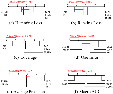
Results on Known Labels. Friedman test [Demˇ sar, 2006] is employed to conduct performance analysis among the comparing approaches, and the result of it is shown in Table 3. As shown in Table 3, the null hypothesis that all the comparing algorithms perform equivalently is clearly rejected in terms of all the evaluation metrics at significance level α = 0.05, Consequently, the Nemenyi test [Demˇ sar, 2006] is adopted to analyse the relative performance among them. For Nemenyi test, the critical difference CD=qα√ k(k+1) 6N =1.0167 (k=5, N=36) with qα=2.728 at significance level α=0.05, where k is the number of algorithms and N (16 × 3) is the number of data sets. The CD diagrams of DLCL w.r.t to the comparing algorithms on each evaluation metric are shown in Figure 1. In each sub-figure, any comparing algorithm whose average rank is within one CD to that of DLCL is connected. Otherwise, any algorithm not connected with DLCL is considered to have significant different performance between them. According to these experimental results, the following observations can be made: 1) The proposed method DLCL significantly outperforms the comparing algorithms in terms of ranking loss, average precision, coverage, and AUC. Besides, DLCL statistically outperforms the comparing algorithms in terms of hamming loss and one error. These results definitely demonstrate the effectiveness of our method on MLL. 2) KRAM and MLkNN algorithms are all constructed based on the information of k nearest neighbors of each instance. It is worth noting that these two algorithms achieve worse performance on those data with a large number of labels (e.g., l≥100) than on those data with a small number of labels. One possible reason might be that the k nearest neighbors can not provide sufficient information for model construction when many labels are hidden in the data. These results verify the importance of discovering latent class labels for MLL.
| Data sets | DLCL (k, q) | RS (.3l, .7l) | ||||
|---|---|---|---|---|---|---|
| (.1l, .9l) | (.2l, .8l) | (.3l, .7l) | r1 | r2 | r3 | |
| arts | .235±.03 | .315±.03 | .265±.01 | .153 | .154 | .155 |
| bibtex | .093±.01 | .197±.01 | .215±.01 | .090 | .087 | .096 |
| corel16k1 | .266±.01 | .265±.01 | .251±.01 | .066 | .066 | .066 |
| corel16k2 | .223±.01 | .240±.01 | .249±.01 | .065 | .080 | .106 |
| corel5k | .094±.01 | .145±.01 | .144±.01 | .129 | .112 | .094 |
| education | .051±.01 | .100±.01 | .123±.01 | .105 | .119 | .118 |
| medical | .163±.02 | .224±.03 | .273±.03 | .148 | .145 | .145 |
| rcv1v2s1 | .182±.02 | .202±.02 | .203±.02 | .094 | .106 | .117 |
| chemistry | .115±.02 | .131±.01 | .149±.01 | .088 | .084 | .086 |
| cooking | .176±.02 | .203±.01 | .229±.01 | .104 | .080 | .073 |
| cs | .146±.01 | .171±.01 | .203±.01 | .089 | .079 | .079 |
| philosophy | .154±.02 | .160±.01 | .192±.01 | .135 | .111 | .102 |
Results on Latent Labels. Table 4 shows the results of DLCL on discovered latent class labels according to Fnovel. It is clearly indicated that DLCL can discover the latent labels for MLL, and DLCL significantly outperforms RS(Randomly Setting) when q = 70l% and k = 30l%. For some data sets, the results of Fnovel differ extremely under different ratios of latent labels. The possible reason might be that the difficulties of prediction of different labels are different. On the other hand, we want to know what latent labels have we discov-
| Matched Label Name | Fnovel | Top 20 Features (i.e., feature name (weight)) |
|---|---|---|
| regular-languages | 0.712 | regular(0.898), beginalign(0.062), endalign(0.052), essenti(0.045), express(0.039), pump(0.036), confus(0.035), project(0.034), home- work(0.034), attempt(0.034), independ(0.032), languag(0.03), let(0.027), digit(0.027), cup(0.026), lot(0.026), comment(0.026), identi- fi(0.026), algebra(0.025), here(0.025) |
| pumping-lemma | 0.635 | pump(0.855), lemma(0.681), essenti(0.139), easier(0.12), identifi(0.1), formul(0.083), split(0.076), condit(0.068), geq(0.068), re- spect(0.067), nice(0.067), forc(0.063), short(0.061), imagin(0.058), author(0.056), larger(0.054), yield(0.054), effect(0.053), pseu- docod(0.053), insid(0.051) |
| reductions | 0.564 | reduct(0.83), beginalign(0.11), endalign(0.099), reduc(0.074), langl(0.065), notic(0.054), show(0.053), sat(0.039), suggest(0.034), shown(0.034), nice(0.031), maxim(0.03), naiv(0.029), undecid(0.029), simpl(0.027), research(0.027), flow(0.026), wikipedia(0.024), wrong(0.024), literatur(0.024) |
| turing-machines | 0.465 | machin(0.829), ture(0.617), tape(0.122), encod(0.041), power(0.038), occur(0.036), simul(0.034), digit(0.031), determinist(0.030), build(0.030), group(0.029), appear(0.029), qquad(0.028), make(0.028), automaton(0.027), uniqu(0.027), troubl(0.027), play(0.026), halt(0.026), endalign(0.026) |
| sorting | 0.448 | sort(0.849), comparison(0.136), insert(0.119), quick(0.061), compar(0.035), addit(0.031), entri(0.030), notat(0.029), origin(0.028), se- lect(0.027), algorithm(0.027), automata(0.027), free(0.026), easi(0.026), sourc(0.026), qquad(0.026), mark(0.026), shown(0.026), dig- it(0.025), argument(0.025) |
k
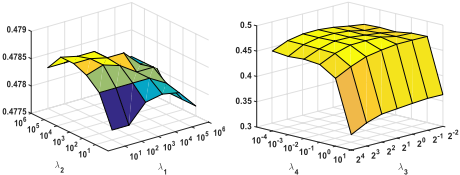
Figure 3: Parameter analysis on DLCL over stackex-chemistry.
ered. We try to describe the meaning of them by the learned labels-specific features which are indicated by the non-zero entities of each column of W. Table 5 shows the results of the five best matched labels over the stackex-cs data set with q = 70l% and k = 30l%. It is noted that the names of top five matched labels are the occurred among the top 20 features or homologous with them, and most of features have a strong semantic correlation with the name of labels.
4.3 Parameter and Convergence Analysis
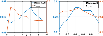
The number of Latent labels k and correlation confidence α. For arts, the first 20 and the rest 6 labels are set as known and latent labels respectively. Figure 2 shows the average results of DLCL over 10 repetitions with different values of k and α. The result (i.e., Macro AUC) on known labels is improved by discovering latent labels (i.e., k > 0), and the Fnovel decreases with the increasing of k. The larger the number of latent labels, the harder it is to discover them. Therefore, we could set k to be a relative small value and run DLCL multiple times. It is also noted that the performance of latent labels can be significantly improved with the help of known labels and the improvement on known labels is slightly with the help of latent labels by exploiting their correlations (i.e., α > 0). The known labels are observed in advance and can be considered as a teacher to guide the prediction on latent labels.
Analysis on regularization parameters. The average results (i.e, Average Precision) of DLCL with different values of λ1, λ2, λ3, and λ4 over stackex-chemistry are shown in Figure 3, and similar results were also obtained for the other data sets. It is noted that the performance of DLCL is insensitive to the parameters, and also the optimal performance is usually achieved at some intermediate values of each parameter.
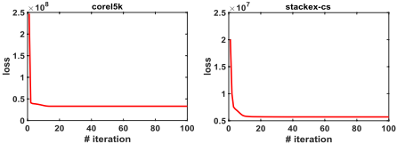
Convergence. Figure 4 demonstrates two examples of the convergence curves of DLCL. It is noted that the values of the objective function are non-increasing and drop sharply around 15 iterations on corel5k and stackex-cs data sets.
5 Conclusion
In this paper, a novel approach named DLCL is proposed for MLL which can not only discover the latent labels in the training data but also predict new instances with these latent labels and known labels simultaneously. The experimental results demonstrate that the performance of latent labels can be significantly improved with the help of known labels and the performance of known labels can be improved with the help of latent labels by exploiting their correlations. Extensive experiments with other state-of-the-art MLL approaches have show a competitive performance of DLCL.
Acknowledgement
This work is supported by JST KAKENHI: 191400000190, JST-AIP: JPMJCR19U4, and NSFC: 61806005.
@inproceedings{ijcai2020p423,
  title     = {Discovering Latent Class Labels for Multi-Label Learning},
  author    = {Huang, Jun and Xu, Linchuan and Wang, Jing and Feng, Lei and Yamanishi, Kenji},
  booktitle = {Proceedings of the Twenty-Ninth International Joint Conference on
               Artificial Intelligence, {IJCAI-20}},
  publisher = {International Joint Conferences on Artificial Intelligence Organization},
  editor    = {Christian Bessiere},
  pages     = {3058--3064},
  year      = {2020},
  month     = {7},
  note      = {Main track},
  doi       = {10.24963/ijcai.2020/423},
  url       = {https://doi.org/10.24963/ijcai.2020/423},
}
TY - CPAPER TI - Discovering Latent Class Labels for Multi-Label Learning AU - Huang, Jun AU - Xu, Linchuan AU - Wang, Jing AU - Feng, Lei AU - Yamanishi, Kenji T2 - Proceedings of the Twenty-Ninth International Joint Conference on Artificial Intelligence, IJCAI-20 PB - International Joint Conferences on Artificial Intelligence Organization PY - 2020 SP - 3058 EP - 3064 DO - 10.24963/ijcai.2020/423 UR - https://doi.org/10.24963/ijcai.2020/423 ER -Copied
Machine-readable versions of this paper, for tools and AI agents:





